Windowing Method to design FIR filters

I know if you’ve made it this far in this Digital Signal Processing course, you might have had a few moments where you’d have thought of jumping out the window. But bear with me and leave the windowing technique to FIR filters. Trust me, it is not as complicated as it seems.

Contents

Introduction to Windowing Method

It would seem straightforward to think that to obtain causal FIR filters we can just truncate the infinite Fourier series of the non-causal Infinite Impulse Response (IIR) filter.

However, in practice, the abrupt nature of the truncation causes oscillations to show up on the passband and stopband of the filtered response. This is also known as Gibb’s phenomenon that we had previously discussed.

The Windowing Technique, in which the windowing function is multiplied with the desired frequency response, helps minimize the effects of these oscillations giving us a more desirable output from the truncation of the IIR filter.

Windowing

But how do you determine the frequency range to ensure you design an effective filter. This is where the windowing technique comes in.

Visualize sending an infinite function into a window to get back a finite part of it that enables us to analyze it with more ease. That is essentially what we are trying to achieve with the Windowing method.

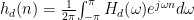
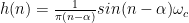
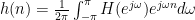
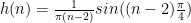
Breaking things down, first, we have to choose a proper frequency-selective IIR filter. This filter usually has a non-causal (has both negative and positive points) and infinite duration impulse response. The specification of the frequency response is usually given in the form of ${ H }_{ d }(\omega )$ . Here is the waveform of the frequency response.

This frequency response should be converted to unit sample response using the Fourier transform relation shown below

${ H }_{ d }(\omega )=\sum _{ n=0 }^{ \infty }{ { h }_{ d }(n){ e }^{ -j\omega n } }$

and

${ h }_{ d }(n)=\frac { 1 }{ 2\pi } { \int _{ -\pi }^{ \pi }{ { H }_{ d }( } \omega ){ e }^{ j\omega n }d\omega }$

Now, we want to send this waveform, ${ h }_{ d }(n)$ , through a window. Basically, truncate the waveform so that we obtain a causal and linear-phase FIR filter (opposite of what we had before, which basically means finite and probably positive). The filter is truncated to a particular length; this length is also known as the window length. Let’s say it is truncated at the point n. Which means the FIR filter length would be M=n+1. Let the rectangular window be w(n), which is given as

$w(n)=1, \quad n=0,1,...M-1\quad ;$ $w(n)=0\quad otherwise$

Let the waveform of w(n) look like this:

Now we are combining the two waveforms, ${ h }_{ d }(n)$ and w(n) to obtain h(n), the unit sample response of the FIR filter.

${ h(n)=h }_{ d }(n)w(n)={ h }_{ d }(n)\quad$ for n=0,1,…,M-1;0 otherwise

Hence, the graph of h(n) would look like this which is basically the convolution of ${ h }_{ d }(n)$ and w(n)

For a bit of perspective, let us take the equation of a linear phase FIR filter where the order M is even.

${ H(e }^{ j\omega })=\sum _{ k=0 }^{ m }{ h[k] } { e }^{ -jk\omega }={ e }^{ -j\omega \frac { m }{ 2 } }A(\omega )$

where $A(\omega)$ is the real magnitude function

We are going to start off by minimizing the mean square error between the actual filter and a desired filter. The coefficient of the actual filter is represented by h[k].

$\begin{matrix} min \\ h[k] \end{matrix}\frac { 1 }{ 2\pi } \int _{ -\pi }^{ \pi }{ { \left| { H }_{ d }({ e }^{ j\omega })-H({ e }^{ j\omega }) \right| }^{ 2 }d\omega }$

where ${ H }_{ d }({ e }^{ j\omega })$ represents the desired response and $H({ e }^{ j\omega })$ represents the actual response

The desired filter is also a linear phase FIR filter with the same group delay, let this equation be represented by

${ { H }_{ d }(e }^{ j\omega })={ e }^{ -j\omega \frac { m }{ 2 } }A_{ d }(\omega )$

where the mean squared error is represented by

$\begin{matrix} min \\ a[k] \end{matrix}\frac { 1 }{ 2\pi } \int _{ -\pi }^{ \pi }{ { \left| { A }_{ d }(\omega )-A(\omega ) \right| }^{ 2 }d\omega }$ –(1)

where $a[k]=h[k+m/2]$ this represents the shift to the left and applying Discrete-time Fourier Transform(DTFT) to a[k] you will obtain $A(\omega)$ .

The Parseval’s theorem (See properties of DFT) states that the integral of the magnitude squared in the frequency domain is equal to the sum of the magnitude squared in the time domain, hence equation(1) can also be written as

$\begin{matrix} min \\ a[k] \end{matrix}\sum _{ k=-\infty }^{ \infty }{ { \left| a_{ d }[k]-a[k] \right| }^{ 2 } }$ –(2)

where a[k] is non-zero for the interval $\frac { -m }{ 2 } \le k\le \frac { m }{ 2 }$

expanding equation(2) we get

$\begin{matrix} min \\ a[k] \end{matrix}\sum _{ k=-\infty }^{ \infty }{ { \left| a_{ d }[k]-a[k] \right| }^{ 2 } } =\sum _{ k=-m/2 }^{ m/2 }{ { \left| a_{ d }[k]-a[k] \right| }^{ 2 } } +\sum _{ k=-\infty }^{ -m/2-1 }{ { \left| a_{ d }[k] \right| }^{ 2 } } +\sum _{ k=m/2+1 }^{ \infty }{ { \left| a_{ d }[k] \right| }^{ 2 } }$

We have to choose a[k] accordingly so that the first term becomes 0, to satisfy that

let $a[k]=a_{ d }[k] for \frac { -m }{ 2 } \le k\le \frac { m }{ 2 }$

This is actually equivalent to multiplying infinite response with a windowing function

$a[k]={ a }_{ d }[k].w[k]$

This is the same as

$A(\omega )={ A }_{ d }(\omega )*W({ e }^{ j\omega })$

Here is a graphical representation of the convolution happening in the above equation

The discrete-time Fourier Transform of $a_{ d }[k]$ which is ${ A }_{ d }(\omega )$

The Rectangular Window function is shown below

Taking the Discrete-time Fourier Transform of the windowing function we get the graph of $W({ e }^{ j\omega })$

This graph by the main lobe having a width of $\frac { 4\pi }{ m+1 }$ . The first peak side of the lobe goes down to -13dB relative to the main lobe.

So, the convolution of the window function and the desired filter’s magnitude response will give us the graph below

As you can see from the graph, there are many isolations and ripples present in the stopband and the passband. The main lobe of the graph of $W({ e }^{ j\omega })$ determines the transition bandwidth and the width of the side lobes determine the passband and stopband ripples.

These ripples are not acceptable for a filter of quality. Too many ripples on the passband and stopband will not let a filter do its function well enough. Typically, other windows are used to trade the main lobe width (transition band) for the sidelobe widths (ripples).

Types of Windows

Type of Window	Windowing Function	Shape of Windowing Function	Widths of Lobes of the frequency response
Rectangular	w(n)=1		Main lobe width= $\frac { 4\pi }{ m+1 }$ Height of Side lobe =-13dB
Bartlett (Triangular)	w(n)=1- $\frac { 2\left\| n-\frac { m }{ 2 } \right\| }{ m }$		Main lobe width= $\frac { 8\pi }{ m }$ Height of Sidelobe =-25dB
Hanning	w(n)=0.5 – 0.5cos $(\frac { 2\pi n }{ m } )$		Main lobe width= $\frac { 8\pi }{ m }$ Height of Sidelobe =-31dB
Hamming	w(n)=0.54 – 0.46cos $(\frac { 2\pi n }{ m } )$		Main lobe width= $\frac { 8\pi }{ m }$ Height of Side lobe =-41dB
Blackman	w(n)=0.42 – 0.5cos $(\frac { 2\pi n }{ m } )$ + 0.08cos $(\frac { 4\pi n }{ m } )$		Main lobe width= $\frac { 12\pi }{ m }$ Height of Side lobe =-57dB
Kaiser	w(n)= $\frac { { I }_{ 0 }\quad \left\{ \beta { \left[ 1-{ \left( \frac { n-\alpha }{ a } \right) }^{ 2 } \right] }^{ 1/2 } \right\} }{ { I }_{ 0 }(\beta ) }$

Advantages and Disadvantages of the Windowing Technique

It is a simple method to implement to get the desired response.
It does not have much flexibility as there are an equal amount of passband and stopband ripples present in the response that limits the ability of the designer to make the output more ideal.
There is minimum computation involved in executing this technique.
No matter how much we increase the value of m, the maximum magnitude of the ripple is fixed (except when using the Kaiser Window.)
Due to the convolution of the desired frequency response and the spectrum of the windowing function, it is not possible to find out the specific values of the passband and the stopband frequencies.
When the filter order, m is increased this leads to a narrower frequency response in which the smoothing is reduced. This leads to big side lobes that are coupled with a lower transition width which is Gibb’s phenomenon that was previously mentioned. However, the Blackman-Harris Window helps to reduce the effects of Gibb’s phenomenon and keep it to a minimum.

Steps for solving problems using the windowing method

Let us look at how to utilize these functions that we have learned about in a problem. First, let us go through the steps to solving a problem relating to the windowing method of FIR filters.

Step 1:

Find out $H(\omega )\quad and\quad { \omega }_{ c }$ $H(\omega )={ e }^{ -j\alpha \omega }$

The equation can be given directly in the equation
The value of m can be given and you have to calculate α=(m-1)/2
The phase delay is given, the value of α, with which you can find out $H(\omega )$

${ \omega }_{ c }$

This value can be given directly
The cutoff frequency, ${ f }_{ c }$ can be given with which you have to find ${ \omega }_{ c }=2\pi { f }_{ c }$
The sampling frequency, ${ F }_{ s }$ can be given with which you have to find ${ \omega }_{ c }=\frac { 2\pi { f }_{ c } }{ { F }_{ s } }$

Step 2:

Now, we find the value of h(n) of the IIR filter response by taking the Inverse Discrete Fourier Transform of $H(\omega )</p> [latex]h(n)=\frac { 1 }{ 2\pi } \int _{ -\pi \pi }^{ \pi }{ H(\omega ){ e }^{ j\omega n }d\omega }$

For a Low Pass Filter,

$h(n)=\frac { 1 }{ \pi (n-\alpha ) } sin(n-\alpha ){ \omega }_{ c }$

For a High Pass Filter,

$h(n)=\frac { -1 }{ \pi (n-\alpha ) } sin(n-\alpha ){ \omega }_{ c }$

You will have to find h(n) for all vales of n based on m

However, when n=α

h(α)= $\frac { 1 }{ 2\pi } \int _{ -\pi }^{ \pi }{ d\omega ({ e }^{ -j\alpha \omega } } { e }^{ j\alpha \omega })$

Hence, the integral term will be cancelled off.

Step3:

Now, you have to identify the windowing function based on what window you are using as you see from the table. Substitute the values of n into the function to get the coefficients pertaining to the window function. You can form a table similar to the one below for better understanding

Value of n	Desired Frequency Response, h_d(n)	Windowing Function, w(n)	Function after performing Windowing method, h(n)= h_d(n). w(n)
0	h_d(0)	w(0)	h(0)= h_d(0). w(0)
1	h_d(1)	w(1)	h(1)= h_d(1). w(1)
. . .	. . .	. . .	. . .
m-1	h_d(m-1)	w(m-1)	h(m-1)= h_d(m-1). w(m-1)

Step 4:

Now, we have to find the final equation after the windowing technique has been applied. To identify which of the values from the table above should be included, you need to solve this equation and substitute the respective values from the table above:

$H({ e }^{ j\omega })=h(\frac { N-1 }{ 2 } )+\sum _{ n=1 }^{ \frac { N-1 }{ 2 } }{ 2h(\frac { N-1 }{ 2 } -n)cos(\omega n) }$

Simplifying and solving this equation will give you the final transfer function

Step 5:

We are not done just yet, we have to transform this final equation using the z-transform into the 'z' domain.

Example using rectangular window

Question

Given the frequency specifications as follows and the information that we are using a rectangular window, find the truncated filter response

${ H }_{ d }({ e }^{ j\omega })=\quad { e }^{ -j2\omega }\quad \quad \frac { -\pi }{ 4 } \le \omega \le \frac { \pi }{ 4 } ;\quad o\quad \quad \quad \omega \le \frac { -\pi }{ 4 } \quad \& \quad \omega \ge \frac { \pi }{ 4 }$

Solution

Taking into account the limits we can graph the frequency like the one shown below

Drawing the waveform, we understand it is a low pass filter as it allows the low-frequency range to pass.

Now apply inverse discrete transform while changing the limits respectively,

$h(n)=\frac { 1 }{ 2\pi } \int _{ -\pi }^{ \pi }{ H({ e }^{ j\omega }){ e }^{ j\omega n } } d\omega$ $h(n)=\frac { 1 }{ 2\pi } [\int _{ -\pi }^{ -\pi /4 }{ H({ e }^{ j\omega }){ e }^{ j\omega n } } d\omega +\int _{ -\pi /4 }^{ \pi /4 }{ H({ e }^{ j\omega }){ e }^{ j\omega n } } d\omega +\int _{ \pi /4 }^{ \pi }{ H({ e }^{ j\omega }){ e }^{ j\omega n } } d\omega ]$

Outside the limits the expressions tend to 0 cancelling of those terms leaving us with

$h(n)=\frac { 1 }{ 2\pi } [\int _{ -\pi /4 }^{ \pi /4 }{ H({ e }^{ j\omega }){ e }^{ j\omega n } } d\omega ]$ $h(n)=\frac { 1 }{ 2\pi } [\int _{ -\pi /4 }^{ \pi /4 }{ { e }^{ -j2\omega }{ e }^{ j\omega n } } d\omega ]$ $h(n)=\frac { 1 }{ 2\pi } [\int _{ -\pi /4 }^{ \pi /4 }{ { e }^{ j(n-2)\omega } } d\omega ]$ $h(n)=\frac { 1 }{ 2\pi } [\frac { { e }^{ j(n-2)\omega } }{ j(n-2) } ]\begin{matrix} \pi /4 \\ -\pi /4 \end{matrix}$ $h(n)=\frac { 1 }{ 2\pi } [\frac { { e }^{ j(n-2)\frac { \pi }{ 4 } } }{ j(n-2) } -\frac { { e }^{ j(n-2)(\frac { -\pi }{ 4 } ) } }{ j(n-2) } ]$

Using the formula $sin\theta =\frac { { { e }^{ j\theta }-e }^{ -j\theta } }{ 2j }$ $h(n)=\frac { 1 }{ \pi (n-2) } sin((n-2)\frac { \pi }{ 4 } )$

This value is an infinite function
Now, in the question we are also given that the windowing function is as shown below

$w(n)=1\quad 0\le n\le 4;\quad 0\quad otherwise$

Therefore, multiplying the windowing function and the unit sample response, we get the truncated filter response as

h'(n)=h(n).w(n)

$h'(n)=\frac { 1 }{ \pi (n-2) } [sin((n-2)\frac { \pi }{ 4 } ].(1)$

Transforming this into the 'z'-plane, we get

$h(z)=\frac { 1 }{ \pi (n-2) } [\frac { sin((n-2)\frac { \pi }{ 4 } )z }{ { z }^{ 2 }{ -2cos((n-2)\frac { \pi }{ 4 } )z+1 } } ]\quad$

So, hope you understand what really is the whole deal with this rectangular window. But, there is more to it. As mentioned, above there are several types of filters that are used to get an optimum response from the filter. The rectangular filter does not do enough as mentioned, it causes many ripples in the passband and stopband.

Also while using the rectangular window, remember how infinite is turned to finite, unfortunately, some information may be lost along with this process as well because the convolution of the two functions may lead to the flattening of the waveform.

This flattening of the waveform can be reduced by increasing the value of M as will get narrower. These discrepancies lead to large side lobes which bring about the ringing effect in the FIR filter and make it inaccurate.

Now hold up, what is this ringing effect? No, it is not the bells you hear when you know you are in trouble during an exam. In fact, it is called Gibb’s phenomenon. It is just a fancy name for the annoying distortions around sharp edges in photos and videos. To avoid this ringing effect we have the other window types that we previously mentioned.

Let us look at a problem where one of the other windowing functions are used so you can understand how to implement them when the window function is not just simply equal to 1.

Example using Hamming window

Question

Design a FIR Filter for the given specification by using a hamming window.

${ H }_{ d }({ e }^{ j\omega })={ e }^{ -3j\omega }\quad \frac { -\pi }{ 4 } \le \omega \le \frac { \pi }{ 4 } ;\quad o\quad otherwise$

Solution

${ h}_{ d }({ e }^{ j\omega })=\frac { 1 }{ 2\pi } \int _{ -\pi }^{ \pi }{ { H }_{ d }({ e }^{ j\omega }) } { e }^{ j\omega n }d\omega$ ${ h}_{ d }({ e }^{ j\omega })=\frac { 1 }{ 2\pi } \int _{ -\pi }^{ \pi }{ { e }^{ -j3\omega } } { e }^{ j\omega n }d\omega$ ${ h}_{ d }({ e }^{ j\omega })=\frac { 1 }{ 2\pi } \int _{ -\pi }^{ \pi }{ { e }^{ j\omega (n-3) } } d\omega$ ${ h }_{ d }({ e }^{ j\omega })=\frac { 1 }{ 2\pi } [\frac { { e }^{ j\omega (n-3) } }{ j\omega (n-3) } ]\begin{matrix} \pi /4 \\ -\pi /4 \end{matrix}$ ${ h }_{ d }({ e }^{ j\omega })=\frac { 1 }{ 2\pi j(n-3) } [{ e }^{ j\frac { \pi }{ 4 } (n-3) }-{ e }^{ -j\frac { \pi }{ 4 } (n-3) }]$

Using the formuals ${ e }^{ j\theta }-{ e }^{ -j\theta }=2jsin\theta$ $\frac { { e }^{ j\theta }-{ e }^{ -j\theta } }{ 2j } =sin\theta$ --(3)

Hence,

${ h }_{ d }(n)=\frac { 1 }{ \pi (n-3) } [sin(\frac { \pi }{ 4 } (n-3)]$

since $0\le n\le m-1$

From 3 we can deduce that α=3

α=(m-1)/2

Therefore, m=7

Find w(n)

For a hamming window, we know the function is

$w(n)=0.5-0.5cos(\frac { 2\pi n }{ m } )$

Calculate h[n] $h[n]={ h }_{ d }[n].w[n]$ $h[n]=\frac { 1 }{ \pi (n-3) } [sin(\frac { \pi }{ 4 } (n-3)].[0.5-0.5cos(\frac { 2\pi 3 }{ 6 } )]$

n=0 to 6 as m=7 and equation becomes 0 when α=3

simplifying h(3), we realise we get an indeterminate value

h(3)=0/0

Hence, applying the L'Hopital Rule

where $\begin{matrix} Let \\ \theta \rightarrow 0 \end{matrix}\quad \frac { sinA\theta }{ \theta } =A$

we can deduce

$h(3)=\begin{matrix} Lt \\ \theta \rightarrow 0 \end{matrix}\quad \frac { sin\frac { \pi }{ 4 } (n-3) }{ \pi (n-3) } =\frac { 1 }{ 4 }$ $h(3)=\frac { 1 }{ 4 } [0.54-0.46cos\pi ]$ $h(3)=\frac { 1 }{ 4 } [0.54-0.46(-1)]$

h(3)=0.25

Figure out the magnitude response

$H({ e }^{ j\omega })=h(\frac { N-1 }{ 2 } )+\sum _{ n=1 }^{ \frac { N-1 }{ 2 } }{ 2h(\frac { N-1 }{ 2 } -n)cos(\omega n) }$ $H({ e }^{ j\omega })=h(3)+\sum _{ n=1 }^{ 3 }{ 2h(3-n)cos(\omega n) }$ $H({ e }^{ j\omega })=h(3)+2h(2)cos\omega +2h(1)cos2\omega +2h(0)cos3\omega$ --(4)

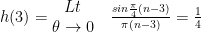
We have calculated for n=3,

it is time to find h(n) for n=0,1,2,4,5,6

h(n)=h(N-1)

Hence, the values will be symmetric

h(0)=h(6)

h(1)=h(5)

h(2)=h(4)

h(3)=0.25

Note: Make sure your calculator is in radian mode while doing these calculations.

So, $h[0]=h[6]=\frac { 1 }{ \pi (0-3) } [sin(\frac { \pi }{ 4 } (0-3)].[0.5-0.5cos(\frac { 2\pi 0 }{ 6 } )]=6.002\times { 10 }^{ -3 }$ $h[1]=h[5]=\frac { 1 }{ \pi (1-3) } [sin(\frac { \pi }{ 4 } (1-3)].[0.5-0.5cos(\frac { 2\pi 1 }{ 6 } )]=0.049$ $h[2]=h[4]=\frac { 1 }{ \pi (2-3) } [sin(\frac { \pi }{ 4 } (2-3)].[0.5-0.5cos(\frac { 2\pi 2 }{ 6 } )]=0.1733$

Now, that we have the values for n=0 to 6 , we can substitute them back into the equation (4) to get

$H({ e }^{ j\omega })=0.25+2(0.173)cos\omega +2(0.049)cos2\omega +2(0.006)cos3\omega$

and your final equation

$H({ e }^{ j\omega })=0.25+0.346cos\omega +0.098cos2\omega +0.012cos3\omega$

Transforming this to the z-plane, we have the final transfer function

$H(z)=0.25+0.346\frac { (1-{ z }^{ -1 }cos(\omega )) }{ { (z }^{ -1 }-{ cos(\omega )) }^{ 2 }+(sin(\omega { )) }^{ 2 } } +0.098\frac { (1-{ z }^{ -1 }cos(2\omega )) }{ { (z }^{ -1 }-{ cos(2\omega )) }^{ 2 }+(sin(2\omega { )) }^{ 2 } } +0.012\frac { (1-{ z }^{ -1 }cos(3\omega )) }{ { (z }^{ -1 }-{ cos(3\omega )) }^{ 2 }+(sin(3\omega { )) }^{ 2 } } \quad \quad.$

This article equips you with all the fundamental knowledge required to solve windowing problems on your own. To get a better hang of it, go ahead and solve some problems.

Sources: 1, 2, 3, 4