Filter Approximation and its types - Butterworth, Elliptic, and Chebyshev

“Nature, like a true poet, abhors abrupt transitions” -Heinrich Heine

Contents

What is Filter approximation and why do we need it?

Yes, nature resists abrupt changes. Spider-Man, tragically, had to learn this the hard way. His girlfriend, Gwen Stacy, died due to whiplash when he tried to save her after Green Goblin throws her off the bridge. The abrupt stop by Spidey’s webbing proved fatal for Gwen. Was there any other way the web-slinger could have done it better?

Perhaps not.

But we definitely can respect nature’s limits to avoid undesirable consequences of abruptness in our DSP system!

To achieve a realizable and a practical filter, we introduce some approximations to the filter design. Let us compare an ideal filter with a practical one:

An ideal “brick wall” filter has:

an abrupt transition from pass-band to stop-band and vice-versa.
no attenuation in pass-band.
infinite attenuation in stop-band.

A practical filter has:

gradual transitions.
non-zero (still, negligible) attenuation in pass-band (pass-band ripple).
doesn’t completely attenuate in stop-band (stop-band ripple).

The cut-off frequencies are the only specifications we needed to define an ideal filter. The practical realization requires a couple or more specs:

Cut-off Frequency ωc
Stopband frequency ωs
Pass-band Ripple 1 − Ap: Amount of variation (fluctuation) in the magnitude response of the filter. You can expect the pass-band frequencies of your signal to be attenuated by a factor within the pass-band ripple.
Stop-band attenuation As is the maximum attenuation to the frequencies in stop-band.

Let us play around with these specs to define different types of approximations.

What are the different types of Filter approximations?

Butterworth filter

As smooth as butter

Yep, Stephen Butterworth was known for solving impossible mathematical problems and he took up the challenge of making the pass-band ripple-free, flat and as smooth as possible.

The gain Gn(ω) on nth-order lowpass Butterworth filter as a function of discrete frequency ω is given as:

${ G }_{ n }{ (\omega ) }^{ 2 }=\frac { 1 }{ 1+{ (\frac { j\omega }{ j{ \omega }_{ c } } ) }^{ 2n } }$

Advantages of Butterworth filter approximation

No pass-band ripple, that means, all pass-band frequencies have identical magnitude response.
Low complexity.

Disadvantages of Butterworth filter approximation

Bad selectivity, not really applicable for designs that require a small gap between pass-band and stop-band frequencies.

Elliptic

As sharp as a whip

Has the sharpest (fastest) roll-off but has ripple in both the pass-band and the stop-band.

The gain for lowpass elliptic filter is given by:

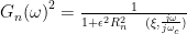
${ G }_{ n }{ (\omega ) }^{ 2 }=\frac { 1 }{ 1+{ { \epsilon }^{ 2 }{ R }_{ n }^{ 2 }\quad (\xi ,\frac { j\omega }{ { j\omega }_{ c } } ) } }$

where, s is the ripple factor derived from pass-band ripple, Rn is known as nth order elliptical rational function and ξ is the selectivity factor derived from stop-band attenuation.

Advantages of Elliptic filter approximation

Best selectivity among the three. Ideal for applications that want to effectively eliminate the frequencies in the immediate neighborhood of pass-band.

Disdvantages of Elliptic filter approximation

Ripples in both the bands and hence, all frequencies experience non-identical changes in magnitude.
Non-linear phase, that leads to phase distortion.
High complexity.

Chebyshev

Jack of all trades, Master of none

Faster roll-off than Butterworth, but not as fast as Elliptical. Ripples in either one of the bands, Chebyshev-1 type filter has ripples in pass-band while the Chebyshev-2 type filter has ripples in stop-band.

The gain for lowpass Chebyshev filter is given by:

${ G }_{ n }{ (\omega ) }^{ 2 }=\frac { 1 }{ 1+{ { \epsilon }^{ 2 }{ T }_{ n }^{ 2 }\quad (\frac { j\omega }{ { j\omega }_{ c } } ) } }$

where, T_n is known as n^th order Chebyshev polynomial.

Advantages of Chebyshev filter approximation

Decent Selectivity
Moderate complexity

Disadvantages of Chebyshev filter approximation

Ripples in one of the bands.
Non-linear phase, that leads to phase distortion.

Matlab coding exercise

Let us use Matlab’s signal processing toolbox to design

6th order Low-pass Butterworth filter with a cut-off frequency of 3 MHz when the signal is sampled at 10 MHz
6th order Low-pass Chebyshev-1 filter with a cut-off frequency of 3 MHz when the signal is sampled at 10 MHz. Pass-band ripple of 5dB.
6th order Low-pass Chebyshev-2 filter with a cut-off frequency of 3 MHz when the signal is sampled at 10 MHz. Stopband attenuation of 40dB.
6th order Low-pass Elliptic filter with a cut-off frequency of 3 MHz when the signal is sampled at 10 MHz. Passband ripple of 5dB and Stopband attenuation of 40dB.

Matlab Code

fc = 3e6; %cut-off frequency
fs = 10e6; %sampling frquency
n = 6; %order of the filter
As = 40; %Stopband attenuation in dB
Rp = 5; %Passband ripple in dB
[b,a] = butter(n,fc/(fs/2)); % . Normalized frequency Wn = fc/(fs/2). Wn should be between 0 and 1/
[h_butter,w_butter] = freqz(b,a,512); %Obtain frequency response using 512-point FFT
[b,a] = cheby1(n,Rp,fc/(fs/2));
[h_cheby1,w_cheby1] = freqz(b,a,512);
[b,a] = cheby2(n,As,fc/(fs/2));
[h_cheby2,w_cheby2] = freqz(b,a,512);
[b,a] = ellip(n,Rp,As,fc/(fs/2));
[h_ellip,w_ellip] = freqz(b,a,512);
figure;
plot(w_butter/pi,20*log10(abs(h_butter)),'lineWidth',1.2); hold on
plot(w_cheby1/pi,20*log10(abs(h_cheby1)),'lineWidth',1.2); hold on
plot(w_cheby2/pi,20*log10(abs(h_cheby2)),'lineWidth',1.2); hold on
plot(w_ellip/pi,20*log10(abs(h_ellip)),'lineWidth',1.2)
ylim([-100 10]);grid on;
xlabel('Normalized Frequency (\times\pi rad/sample)')
ylabel('Magnitude (dB)')
legend('Butterworth','Chebyshev1','Chebyshev2','Elliptic','FontSize',10)
figure;
plot(w_butter/pi,unwrap(angle(h_butter)),'lineWidth',1.2); hold on
plot(w_cheby1/pi,unwrap(angle(h_cheby1)),'lineWidth',1.2); hold on
plot(w_cheby2/pi,unwrap(angle(h_cheby2)),'lineWidth',1.2); hold on
plot(w_ellip/pi,unwrap(angle(h_ellip)),'lineWidth',1.2); hold on
grid on;
xlabel('Normalized Frequency (\times\pi rad/sample)')
ylabel('Phase (radians)')
legend('Butterworth','Chebyshev1','Chebyshev2','Elliptic','FontSize',10)

Outputs

magnitude response of different filter approximation techniques — Magnitude response

phase response of different filter approximation techniques — Phase response

Observations

Butterworth is the smoothest.
Elliptical is the sharpest.
Chebyshev-2 fails to achieve the desired cut-off frequency at the order of 6. A higher-order (complexity) is needed.
Non-linearity in phase is considerable in Chebyshev and elliptical. Butterworth isn’t completely linear either but it is make do.

One thought on “Filter Approximation and its types – Butterworth, Elliptic, and Chebyshev”

Franklin White says:

April 23, 2020 at 12:48 AM

Wow, I had no idea that Butterworth filters aren’t very complex. That’s great for anyone who is trying to get into using filters. Maybe they aren’t an expert on it yet so they could use a less complex one like a Butterworth filter.