Bilinear transform method of designing IIR filters

Next up, we are going to be learning about another method that can be used to design Digital IIR Filters. So far, we have seen the impulse invariance and Approximation of derivatives methods to design IIR filters. But there are many limitations to these two methods. These methods can only be used to realize low pass filters and a limited class of band-pass filters. We can’t design high pass filters or certain band-reject filters using these two methods. Moreover, the many to one mapping in the impulse invariance method (s-domain to z-domain) causes the issue of aliasing, which is highly undesirable. Bilinear transform removes that issue by using one-to-one mapping. Let’s check out the method.

Contents

What is the Bilinear Transform Method for designing IIR filters?

BLT differs from the rest of the two methods primarily when it comes to the method of mapping from the ‘s’ plane to the ‘z’ plane.
In Bilinear Transformation, we carry out conformal mapping in which the jΩ axis is mapped onto the unit circle in the ‘z’ plane. This is a one-to-one mapping that does not bring along with it the issue of aliasing.
All points in the left-hand side of the s-plane get mapped inside the unit circle in the z-plane. And all points in the right-hand side of the s-plane get mapped outside the circle in the z-plane.
First, we will transform an analog filter, get H(z), and then get a relationship between s and z.
The resulting mapping between the s and z plane will cause a frequency distortion that we will see below. Then we will be carrying out pre-warping to get rid of the effects of frequency warping.

Let us assume an analog filter with the transfer function H(S), where

$H(s)=\frac { b }{ s+a }$ —(1)

Applying the Laplace transform to change the equation from the ‘s’ domain to the time domain, we get

$\frac { dy(t) }{ dt } +ay(t)=bx(t)$ —(2)

y(t) can also be expressed in terms of the equation below

$y(t)=\int _{ { t }_{ O } }^{ t }{ { { y }'(\tau )d\tau +y({ t }_{ O } } } )$ —(3)

As the result of the integral gives us,

$y(t)=y(t)-y({ t }_{ O })+y({ t }_{ O })$

The integral can also be solved by using the trapezoidal rule for finding the area,

Let us say we have a trapezoid of lengths a and b and a height h

The area is given by $A=\frac { a+b }{ 2 } .h$ —(4)

Similarly,

Using the trapezoidal rule(4), the area of the graph between t and tO is given by,

$A=\frac { y'(nT)+y'(nT-T) }{ 2 } .(t-{ t }_{ O })$ —(5)

Where t-t_O is the same as nT-(nT-T) which gives us T

Hence, substituting equation (5) into equation (3), we get

$y(nT)=\frac { T }{ 2 } [y'(nT)+y'(nT-T)]+y({ t }_{ O })$ —(6)

Hold on to that equation for a minute, and let us rearrange equation(2) as shown and

$y'(nT)=-ay(nT)+bx(nT)$ —(7)

Substitute equation(6) into equation(7)

Change y(nT)->y(n) and x(nT)->x(n)

$y(n)=\frac { T }{ 2 } [-ay(n)+bx(n)-ay(n-1)+bx(n-1)]+y(n-1)$

Simplifying the equation by factoring,

$[1+\frac { T }{ 2 } a]y(n)-[1-\frac { T }{ 2 } a]y(n-1)=\frac { bT }{ 2 } [x(n)+x(n-1)]$ —(8)

Applying Z-Transform to the difference equation(8),

y(n)->Y(Z) y(n-1)->Z-1Y(Z)

x(n)->X(Z) x(n-1)->Z-1X(Z)

$[1+\frac { aT }{ 2 } -(1-\frac { aT }{ 2 } ){ Z }^{ -1 }]Y(Z)=\frac { bT }{ 2 } (1+{ Z }^{ -1 })X(Z)$

Arranging this to get a transfer function(output over input->Y(Z) over X(Z)) for the IIR Digital Filter,

$H(Z)=\frac { Y(Z) }{ X(Z) } =\frac { \frac { bT }{ 2 } (1+{ Z }^{ -1 }) }{ 1+\frac { aT }{ 2 } -{ Z }^{ -1 }(1-\frac { aT }{ 2 } ) }$ —(9)

Simplifying this equation,

$H(Z)=\frac { \frac { bT }{ 2 } (1+{ Z }^{ -1 }) }{ 1-{ Z }^{ -1 }+\frac { aT }{ 2 } (1+{ Z }^{ -1 }) }$ $H(Z)=\frac { b }{ \frac { 2 }{ T } (\frac { 1-{ Z }^{ -1 } }{ 1+{ Z }^{ -1 } } )+a }$ —(10)

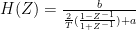
Comparing equation(10) with equation(1),

We can infer that , $s=\frac { 2 }{ T } (\frac { 1-{ Z }^{ -1 } }{ 1+{ Z }^{ -1 } } )$ —(11)

This is the basis of the Bilinear Transformation.

Bilinear Approximation

Here is a little trick.

All the points on the left-hand side(LHS) of the ‘s’ plane are mapped to points inside the unit circle in the ‘z’ plane.
All the points on the right-hand side of the ‘s’ plane are mapped to points outside the unit circle.
All points on the imaginary axis of the ‘s’ plane are mapped points right on the unit circle.

Here’s some context as to why this is the case.

So we know that $Z={ e }^{ sT }$ and $s=\alpha +j\omega$

Joining the two equations together, we have $Z={ e }^{ (\alpha +j\omega )T }$

Ignoring T for just a bit, we can also write Z as $Z={ e }^{ \alpha }{ e }^{ j\omega }$

Mapping the point 0+j0 of the ‘s’ plane onto the ‘z’ plane is when Z=e0=1

Hence, it will fall write on the unit circle as shown in the picture below

Mapping of points onto the unit circle in the z-plane

Based on Euler’s formula,

${ e }^{ j\omega }=cos\omega +jsin\omega$

Hence, taking the modulus would give us

$\left| cos\omega +jsin\omega \right| =\sqrt { { cos }^{ 2 }\omega +{ sin }^{ 2 }\omega } =1$

Hence, the second exponential will always be equal to 1 giving us

$Z={ e }^{ \alpha }1$

So, the value of alpha determines whether the point lies outside or inside the unit circle.

For α <0

Z will also be less than 0 as e to the power of a negative value would give us a value less than 1, mapping the point within the unit circle.

Mapping of points inside the unit circle in the 'z' plane — Mapping of points inside the unit circle in the ‘z’ plane

For α>0

Z will also be greater than 0 as e to the power of a positive value is always greater than 1, mapping the point outside the unit circle.

Mapping of point outside the unit circle of 'z' plane — Mapping of point outside the unit circle of ‘z’ plane

Relationship between Ω and ω

Further investigating the characteristics of Bilinear Transformation, we can actually form an equation relating Ω and ω.

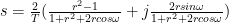
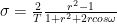
The Z plane expressed in its polar form is

$Z=r{ e }^{ j\omega }$ —(12)

and $s=\alpha +j\omega$ —(13)

Visiting the difference equation that we derived(11) and substituting (12) for all Z.

$s=\frac { 2 }{ T } (\frac { 1-{ Z }^{ -1 } }{ 1+{ Z }^{ -1 } } )$ $s=\frac { 2 }{ T } \frac { r{ e }^{ j\omega }-1 }{ r{ e }^{ j\omega }+1 }$

Remember the euler formula we used before, we’re going to use it again over here and get

$s=\frac { 2 }{ T } \frac { r(cos\omega +jsin\omega )-1 }{ r(cos\omega +jsin\omega )+1 }$

Rationalising the equation above, we obtain

$s=\frac { 2 }{ T } (\frac { { r }^{ 2 }-1 }{ 1+{ r }^{ 2 }+2rcos\omega } +j\frac { 2rsin\omega }{ 1+{ r }^{ 2 }+2rcos\omega } )$ —(14)

Comparing equation(13) with equation(14), we can equate

$\Omega =\frac { 2 }{ T } \frac { 2rsin\omega }{ 1+{ r }^{ 2 }+2rcos\omega }$ —(15)

$\sigma =\frac { 2 }{ T } \frac { { r }^{ 2 }-1 }{ 1+{ r }^{ 2 }+2rcos\omega }$ —(16)

If r value is less than 1, a number less than 1 subtracted by 1(numerator) would give a negative value, hence r<1->σ<1

Similarly, when r is a value greater than 1, a number greater than 1 subtracted by 1(numerator) would give a positive value, hence r>1->σ>1

When r is equal to 1 however, 1 subtracted by 1 would give us σ=0

Hence, simplifying equation(15) and equation(16)

$\Omega =\frac { 2 }{ T } \frac { sin\omega }{ 1+cos\omega } =\frac { 2 }{ T } tan(\frac { \omega }{ 2 } )$ —(17)

$\omega ={ 2tan }^{ -1 }\frac { \Omega T }{ 2 }$ —(18)

Frequency Warping

For an analog filter, the frequency of the filter and the sampling frequency can help find the value of ω.

$\omega =\frac { 2\pi F }{ { F }_{ S } } =\Omega T$

Here we see that there is a linear relationship between Ω and ω.

But, the relationship we determined through the Bilinear Transformation in equation (18) is non-linear.

Frequency Response when there is Frequency Warping

This change in properties when using Bilinear Transformation is referred to as Frequency Warping. The non-linear relationship between Ω and ω results in a distortion of the frequency axis, as seen in the above plot. The spectral representation of frequency using Bilinear Transformation differs from the usual representation.

Is the concept still a little murky? How about an example to help us understand what’s really going down here?

Example

Let us say we have to design a digital IIR filter of cutoff frequency 500Hz and sampling frequency 10KHz.

FC=500Hz and FS=10KHz

ΩC=2πFC=2πx500=1000π=3141.59

ωC=2πFC/FS=1000π/(10x103t)=0.1π=0.314159(Required Cutoff Frequency)

$\hat { { \omega }_{ C } } =2{ tan }^{ -1 }(\frac { { \Omega }_{ C }T }{ 2 } )=2{ tan }^{ -1 }(\frac { 3141.59\times 0.1\times { 10 }^{ -3 } }{ 2 } )=0.3116$ (Mapped Cutoff Frequency after Bilinear Transformation)

Therefore,

${ \omega }_{ C }=\hat { { \omega }_{ C } }$

This change in the frequency value right here is Frequency warping. If we design an analog filter with ωC and then perform Bilinear Transformation and get ${ \omega }_{ C }$ in the digital domain, we cannot design an accurate filter with the same frequency requirement.

Pre-warping

Wait, hold up. You can remove the warping problem using a simple technique. All you have to do to get a digital IIR filter with the same desired cutoff frequency as ωC is to design an analog filter with a cutoff frequency that maps to ωC after Bilinear Transformation. We call this process Pre-warping. We need to pre-warp the analog filters.

Look at the graph we have above, the blue line represents the frequency response after Bilinear Transformation, and the red line represents the Linear characteristics of Ω and ω. To obtain the expected response, which is the red line, we are going to merge the blue line with the green line so that it cancels out and gives us the red line. This is basically what pre-warping does.

How exactly do we calculate this,

With Bilinear Transformation: $\Omega =\frac { 2 }{ T } tan(\frac { \omega }{ 2 } )$

During Prewarping: 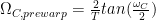${ \Omega }_{ C,prewarp }=\frac { 2 }{ T } tan(\frac { { \omega }_{ C } }{ 2 } )$

Where ωC is the Required Cutoff Frequency

Time for another example, actually the same example as before:

Let us say ωC=0.1π,

Hence, ${ \Omega }_{ C,prewarp }=\frac { 2 }{ T } tan(\frac { { \omega }_{ C } }{ 2 } )={ 2\times 10 }^{ 4 }\times (\frac { 0.1\pi }{ 2 } )=3167.689$

Now, this is the value that we design the analog filter with.

$\hat { { \omega }_{ C } } =2{ tan }^{ -1 }(\frac { { \Omega }_{ C,prewarp }\times T }{ 2 } )=2{ tan }^{ -1 }(\frac { 3167.689\times { 10 }^{ -4 } }{ 2 } )=0.314159=0.1\pi$

After pre-warping, we see that the mapped cutoff frequency is the same as that of the required cutoff frequency. Hence, pre-warping is used to ensure we have the same cutoff frequency for both the analog filter and the digital IIR filter redeeming Bilinear Transformation for us.

Now, is it necessary to go through so much trouble and perform Bilinear Transformation, why not just go with the other two methods?

How about we discuss the pros and cons of this method before coming to any conclusions?

What are the advantages of the Bilinear Transformation method for designing IIR filters?

The mapping is purely one-to-one. While it is not necessarily the same with impulse invariance method.
There is no bother of the aliasing effect.
A stable analog filter can be transformed into a stable digital filter
There are no restrictions on the type of filters that can be transformed. While the other two methods are limited to Low Pass Filters and an even more limited class of Bandpass filters.
There is one to one transformation from the ‘s’ plane to the ‘z’ plane.
All characteristics of the amplitude response of the analog filter are preserved when designing the digital filter. Consequently, the pass band ripple and the minimum stop band attenuation are preserved.

What are the disadvantages of the Bilinear Transformation method for designing IIR filters?

Frequency Warping is the only disadvantage, as the mapping is non-linear we have to perform prewarping.

What is the difference between the Bilinear Transform and Impulse Invariance methods?

Impulse Invariance	Bilinear Transformation
Is used to design IIR filters with the unit sample response represented as h(n) which is obtained by sampling the impulse response of an analog filter	Is used to design IIR filters using the trapezoidal rule in place of numerical integration to get an equation that represents s in terms of Z
The value selected for T is small to reduce the effects of aliasing.	Bilinear Transformation avoids aliasing of frequency components as it is a single conformal mapping of the jΩ axis into the unit circle in the z plane.
Used to design Low pass and a limited class of Band pass IIR Digital filters	Can be used to design all kinds of IIR Digital filters including Low Pass filters, High Pass filters, Band pass, and Band stop filters.
The frequency relationship is linear	Frequency warping takes place as the frequency relationship is non-linear.
Though all poles are mapped from the s-plane to the z-plane, the zeros do not satisfy the same relationship	All zeros and poles are mapped

Solved example using Bilinear Transformation

Given 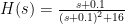$H(s)=\frac { s+0.1 }{ ({ s+0.1) }^ { 2 }+16 }$ and ${ \omega }_{ r }=\frac { \pi }{ 2 }$ . Find H(z)?

Solution

We know that 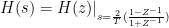$H(s)=H(z){ | }_{ s=\frac { 2 }{ T } (\frac { 1-{ Z }^{ -1 } }{ 1+{ Z }^{ -1 } } ) }$

Comparing the given H(s) equation with the Laplace Transform equation below

$H(s)=\frac { s+a }{ { (s+a) }^{ 2 }+{ { \Omega }_{ C } }^{ 2 } }$

we can deduce that ${ \Omega }_{ C }=4rad/sec$

The relation between Ω and ω as derived above is

${ \Omega }=\frac { 2 }{ T } tan\frac { \omega }{ 2 }$

Therefore, to find T

$T=\frac { 2 }{ { \Omega }_{ C } } tan\frac { { \omega }_{ r } }{ 2 }$ $T=\frac { 2 }{ 4 } tan\frac { \pi }{ 4 }$

hence, T=1/2 secs

Substituting this,

$H(s)=H(z){ | }_{ s=\frac { 2 }{ \frac { 1 }{ 2 } } (\frac { 1-{ Z }^{ -1 } }{ 1+{ Z }^{ -1 } } ) }$

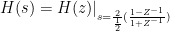
Substituting s in term of z,

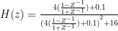
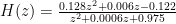
$H(z)=\frac { s+0.1 }{ { (s+0.1) }^{ 2 }+16 } { | }_{ s=\frac { 2 }{ 1/2 } (\frac { 1-{ Z }^{ -1 } }{ 1+{ Z }^{ -1 } } ) }$ $H(z)=\frac { 4(\frac { 1-{ Z }^{ -1 } }{ 1+{ Z }^{ -1 } } )+0.1 }{ { (4(\frac { 1-{ Z }^{ -1 } }{ 1+{ Z }^{ -1 } } )+0.1) }^{ 2 }+16 }$ $H(z)=\frac { \frac { 4(1-{ z }^{ -1 })+0.1(1+{ z }^{ -1 }) }{ (1+{ z }^{ -1 }) } }{ \frac { [4(1-{ z }^{ -1 })+0.1(1+{ z }^{ -1 })]^{ 2 }+16(1+{ z }^{ -1 })^{ 2 } }{ (1+{ z }^{ -1 })^{ 2 } } }$ $H(z)=\frac { 4(1-{ z }^{ -1 })+0.1(1+{ z }^{ -1 }) }{ [4(1-{ z }^{ -1 })+0.1(1+{ z }^{ -1 })]^{ 2 }+16(1+{ z }^{ -1 })^{ 2 } }$ $H(z)=\frac { 0.128{ z }^{ 2 }+0.006z-0.122 }{ { z }^{ 2 }+0.0006z+0.975 }$

Conclusion

We hope you understood the technique of Bilinear Transformation, along with its effects and properties, and pre-warping. This is an important method for designing digital IIR filters. As always, your comments and queries are welcome in the comments section below.

Sources: 1, 2, 3

2 thoughts on “Bilinear transform method of designing IIR filters”

BLTR says:

November 17, 2020 at 10:50 AM

Hi.
That was a really good explanation.
Can you please help me to solve the below question:

A Butterworth LPF of fourth order and cut-off frequency of 1KHz is to be designed.
Sampling frequency is 10 KHz. Transform this filter into discrete time domain by
bilinear transformation such that the resulting filter preserves the gain at 1 KHz. Find
H(z), its poles and zeros.

B L Thulashiramu

Moderator: Comment edited to remove personal email address

BLTR says:

November 17, 2020 at 10:42 AM

Hai Keerthana Jaikumar,
Your explanation was really good. Can you please help me in getting solution for these Questions :

1.)A Butterworth LPF of fourth order and cut-off frequency of 1KHz is to be designed.
Sampling frequency is 10 KHz. Transform this filter into discrete time domain by
bilinear transformation such that the resulting filter preserves the gain at 1 KHz. Find
H(z), its poles and zeros.

For you info, I am also from VIT. Request to give the solution with explanation

Thanks and regards
B L ThulashiRamu

Moderator: Comment edited to remove personal email address and contact number