The Impulse Invariance Method is used to design a discrete filter that yields a similar frequency response to that of an analog filter. Discrete filters are amazing for two very significant reasons:
- You can separate signals that have been fused and,
- You can use them to retrieve signals that have been distorted.
We can design this filter by finding out one very important piece of information i.e., the impulse response of the analog filter. By sampling the response we will get the time-domain impulse response of the discrete filter.
When observing the impulse responses of the continuous and discrete responses, it is hard to miss that they correspond with each other. The analog filter can be represented by a transfer function, Hc(s).
Zeros are the roots of the numerator and poles are the roots of the denominator. For every pole of the transfer function of the analog filter, it can be mapped to a pole on the transfer function of the IIR filter’s transfer function given by H(z). Let us delve deeper into how we can go about doing this.
Contents
Mapping from s-plane to z-plane
The transfer function of the analog filter in terms of partial fraction expansion with real coefficients is

Where A are the real coefficients and P are the poles of the function
And k can be 1, 2 …N.
h(t) is the impulse response of the same analog filter but in the time domain. Since ‘s’ represents a Laplace function Hc(s) can be converted to h(t), by taking its inverse Laplace transform.
Using this transformation,
We obtain
However, in order to obtain a discrete frequency response, we need to sample this equation. Replace ‘nTS’ in the place of t where TS represents the sampling time. This gives us the sampled response h(n),
Now, to obtain the transfer function of the IIR Digital Filter which is of the ‘z’ operator, we have to perform z-transform with the newly found sampled impulse response, h(n). For a causal system which depends on past(-n) and current inputs (n), we can get H(z) with the formula shown below

We have already obtained the equation for h(n). Hence, substitute eqn (2) into the above equation
![H(Z)=\sum _{ n=0 }^{ \infty }{ \left[ \sum _{ k=1 }^{ N }{ { A }_{ k }{ e }^{ { P }_{ K }n{ T }_{ S } } } \right] { Z}^{ -n } }](https://s0.wp.com/latex.php?latex=+H%28Z%29%3D%5Csum+_%7B+n%3D0+%7D%5E%7B+%5Cinfty%C2%A0+%7D%7B+%5Cleft%5B+%5Csum+_%7B+k%3D1+%7D%5E%7B+N+%7D%7B+%7B+A+%7D_%7B+k+%7D%7B+e+%7D%5E%7B+%7B+P+%7D_%7B+K+%7Dn%7B+T+%7D_%7B+S+%7D+%7D+%7D%C2%A0+%5Cright%5D+%7B+Z%7D%5E%7B+-n+%7D+%7D&bg=ffffff&fg=000&s=0&c=20201002)
Factoring the coefficient and the common power of n

Based on the standard summation formula, (3) is modified and written as the required transfer function of the IIR filter.
Hence (4) is obtained from (1), by mapping the poles of the analog filter to that of the digital filter.

That is how you map from the s-plane to z-plane
Relationship of S-plane to Z plane
We had seen a short passage on the mapping from an s-plane to a z-plane in our post discussing the relationship between Z-transform and Laplace transform. We’ll now get into a some specifics for the same.
From the equation above, Since, the poles are the denominators we can say 
Comparing (1) and (4), we can derive that

and since

where
TS is the sampling time
Now, s is taken to be the Laplace operator

σ is the attenuation factor
Ω is the analog frequency
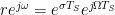
Changing Z from rectangular coordinates to the polar coordinates, we get:

where r is magnitude and ω is digital frequency
Replacing (7) in place of s in (6), and replacing that value as Z in (8)
Compare the real and imaginary parts separately. Where the component with ‘j’ is imaginary.

and

Hence, we can make the inference that

To understand the relationship between the s-plane and Z-plane, we need to picture how they will be plotted on a graph. If we were to plot (7) in the ‘s’ domain, σ would be the X-coordinates and jΩ would be the Y-coordinate. Now, if we were to plot (8) in the ‘Z’ domain, the real portion would be the X-coordinate, and the imaginary part would be the Y-coordinate.
Let us take a closer look at equation (9),
There are a few conditions that could help us identify where it is going to be mapped on the s-plane.
Case 1
when σ <0, it would translate that r is the reciprocal of ‘e’ raised to a constant. This will limit the range of r from 0 to 1.
Since σ <0, it would be a negative value and would be mapped on the left-hand side of the graph in the ‘s’ domain
Since 0<r<1, this would fall within the unit circle which has a radius of in the ‘z’ domain.
Case 2
When σ =0, this would make r=e0, which gives us 1, which means r=1. When the radius is 1, it is a unit circle.
Since σ =0, which indicates the Y-axis of the ‘s’ domain.
Since r=1, the point would be on the unit circle in the ‘z’ domain.
Case 3
When σ>0, since it is positive, r would be equal to ‘e’ raised to a particular constant, which means r would also be a positive value greater than 1.
Since σ>0, the positive value would be mapped onto the right-hand side of the ‘s’ domain.
Since r>1, the point would be mapped outside the unit circle in the ‘z’ domain.
Here is a pictorial representation of the three cases:


Disadvantages of Impulse Invariance Method
- Digital frequency represented by ‘ω,’ and its range lies between – π and π. Analog frequency is represented by ‘Ω,’ and its range lies between – π/TS and π/TS. When mapping from digital to analog, from – π/TS and π/TS , ‘ω’ maps from – π to π. This would make the range of Ω (k-1)π/TS and (k+1)π/TS, where k is an arbitrary constant. However, mapping the other way, from analog to digital, will mean ω maps from – π to π, which makes it many-to-one. Hence, mapping is not one-to-one. This is the main disadvantage.
- Analog filters do not have a definite bandwidth because of which when sampling is performed, this would give rise to aliasing. Aliasing is when the signal eats up into the next signal and so on. This would lead to considerable distortion of the signal. Hence, making the frequency response of the converted digital signal very different from the original frequency response of the analog filter.
- Increasing the sampling time will result in a frequency response that is more spaces out hence decreasing the chances of aliasing. However, this is not the case with this method. Increasing the sampling time has no effect on the amount of aliasing that happens.
- It’s not possible to design a high pass filter using the impulse invariance method.
Steps to design a digital IIR filter using Impulse Invariant Method
- First, we have to obtain H(s), the frequency transfer function of the analog filter. It would either be given directly, or you have to find out the ratio of the output over the input of the filter.
- If it cannot be mapped to the Z-transform as it is, try breaking it down using partial fractions.
- Now, find out the z-transform of each term of the partial fraction expansion.
- You will have your transfer function in terms of H(z), which is the frequency transfer function of the IIR digital filter.
How about we try an example to make sure you get the hang of it?
Solved example using Impulse Invariance method to find the transfer function of an IIR filter
Problem:
Given 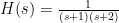
Solution:
Step 1:
Step 2:
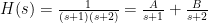
Applying partial fractions on H(s),


Step 3:

Step 4:

That is how you obtain the transfer function of the IIR digital filter.
Try out more questions to get a hang of solving these problems. Once you do that, the impulse invariance method is pretty straightforward. Two points that we should remember before going to the next topic are that the Impulse Invariance method is used for frequency-selective filters and that they are used to transform analog filter design.
