Butterworth Filter Approximation - Impulse Invariance & Bilinear Transform

As discussed in the post on ideal filter types, the Butterworth filter is a filter approximation technique that is also known as the maximally flat filter technique. This filter gives a very flat frequency response in the Pass Band, which ensures that there are no ripples present. Hence, as the name suggests, the maximal flat response you get with the Butterworth Filter cannot be matched by the Chebyshev, Inverse Chebyshev, or Bessel Filters. Though it may not be as effective as the other filters in giving a filter response with a steep transition band, it has a better tolerance to overshoot or ringing compared to the Chebyshev filters. It also allows for minimum attenuation in the Stop Band.

Hence, The Butterworth filter’s applications include:

Anti-Aliasing Filter for Data Converter applications due to its maximally flat nature.
High-quality audio applications as they ensure the frequencies that are supposed to pass do so entirely owing to the flat response, ensuring we hear everything we are supposed to from audio samples.
In motion analysis, digital Butterworth filters are used as they have close to zero ringing in the passband, which gives a clear video for precise analysis.

In this post, we will study the steps for Butterworth Filter approximation and design analog and digital Butterworth filters using the impulse invariance and bilinear transform techniques to design IIR filters.

Contents

Introduction to Butterworth Filters

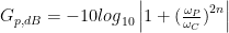
Let us examine a Low Pass Butterworth Filter. The amplitude response of a low-pass Butterworth filter is:

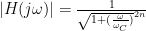
$\left| H(j\omega ) \right| =\frac { 1 }{ { \sqrt { 1+(\frac { \omega }{ { \omega }_{ C } } ) } }^{ 2n } }$

where ${ \omega }_{ C }$ is the filter’s cutoff frequency and n is the order of the filter.

Amplitude Response of Butterworth Filter

The graph you see above represents the magnitude of the frequency response of the filter. From the graph, we can infer that at low frequencies, the gain is very close to 1. But as the frequency increases, the gain goes off and starts rejecting higher frequency components as general low pass filters do. The colors that denote the different values for n are signifying the filter order. Observe that when the filter order is low, the graph rolls off smoothly. However, when the filter order is high, it almost looks like a step function. Hence, we can conclude that to get a smaller transition band, we have to increase the order of the filter.

To simplify the process of designing the Butterworth filter, we are going to be observing a normalized filter first. Then we will be scaling the values to our desired cutoff.

Normalized Butterworth Filter

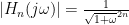
A normalised filter is one that has cutoff frequency equal to 1 ( ${ \omega }_{ C }=1$ )

Hence, the amplitude response will become

$\left| { H }_{ n }(j\omega ) \right| =\frac { 1 }{ { \sqrt { 1+\omega } }^{ 2n } }$

When we square the magnitude of an equation, it is also equal to the magnitude itself multiplied by its complex conjugate. We will be using this property to help with factoring.

${ \left| { H }_{ n }(j\omega ) \right| }^{ 2 }={ H }_{ n }(j\omega ){ H }_{ n }(-j\omega )=\frac { 1 }{ 1+{ \omega }^{ 2n } }$

The transfer function of a filter is given by H(s) which is the impulse response of a filter in the s-domain where $s=\sigma +j\omega$

The frequency response of a filter can be determined by evaluating using the imaginary axis when $s=j\omega$ and $\sigma =0$

The inverse is also possible, given $H(j\omega )$ , you can evaluate H(s) by substituting $\omega =s/j$

Therefore, we can infer

${ \left| { H }_{ n }(j\omega ) \right| }^{ 2 }={ H }_{ n }(j\omega ){ H }_{ n }(-j\omega )={ H }_{ n }(s){ H }_{ n }(-s)=\frac { 1 }{ 1+{ (s/j) }^{ 2n } }$

The 2n denotes the poles of ${ H }_{ n }(s){ H }_{ n }(-s)$ which occur when ${ (s/j) }^{ 2n }=-1$

Putting it in terms of s we get, ${ s }^{ 2n }=-{ (j) }^{ 2n }$ —(1)

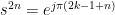
-1 can also be represented in terms of an exponential function as shown

$-1={ e }^{ j\pi (2k-1) }$ , where for every integer k, $j={ e }^{ j\pi /2 }$

So, substituting for the -1 in equation(1)

${ s }^{ 2n }={ e }^{ j\pi (2k-1+n) }$

Taking 1/2n root on each side,

${ s }_{ K }={ e }^{ j\pi (2k+n-1) }=cos(\frac { \pi }{ 2n } (2k+n-1))+jsin(\frac { \pi }{ 2n } (2k+n-1))$

for k=1, 2, 3,…,2n

As you can see from the image above, depending on the value of n the number of poles on each side of the plane will correspond. For example, if N=4, there are four poles in the left-hand plane which correspond to Hn(s), which suggests a causal and stable filter. The four poles on the right-hand plane correspond to the conjugate. Therefore, the number of poles on each side depends on n.

The transfer function for a Normalized Butterworth filter is

${ H }_{ n }(s)=\frac { 1 }{ (s-{ s }_{ 1 })(s-{ s }_{ 2 })...{ (s-s }_{ n }) } =\frac { 1 }{ { s }^{ n }+{ a }_{ n-1 }{ s }_{ n-1 }+...+{ a }_{ 1 }s+1 } =\frac { 1 }{ { B }_{ n }(s) }$

where you obtain the nth order Butterworth polynomial.

${ H }_{ n }(s)$ can be computed by working it out or using a Butterworth Lookup Table, we will look into this in detail while solving the problems.

Scaling Normalized Filter

Now, we know the transfer function for a normalized filter. What if we want a cutoff frequency other than unity?

Depending on the type of filter we would be designing, we would replacing s by the respective transformations shown below to find H(s)

Type of transformation	Transformation(Replace s by the following)
Low Pass	$\frac { s }{ { \omega }_{ C } }$
High Pass	$\frac { { \omega }_{ C } }{ s }$
Band Pass	$\frac { { s }^{ 2 }+{ \omega }_{ l }{ \omega }_{ h } }{ s({ { \omega }_{ h } }-{ \omega }_{ l }) }$
Band Stop	$\frac { s({ { \omega }_{ h } }-{ \omega }_{ l }) }{ { s }^{ 2 }+{ \omega }_{ l }{ \omega }_{ h } }$

where ${ \omega }_{ C }$ is the cutoff frequency

${ \omega }_{ l }$ is the lower band edge frequency

${ \omega }_{ h }$ is the higher band edge frequency

We also need to have specifications of the gain definitions, there are specifically four values that we have to define which can be obtained from the graph below.

Graph to identify Gain definition of a Low Pass Filter

Here

${ G }_{ P }$ is the Pass band gain at Pass band frequency ${ \omega }_{ P }$
${ G }_{ S }$ is the Stop band gain at Stop band frequency ${ \omega }_{ S }$

From these filter specifications, we can determine the order of the filter. The gain is usually represented in dB.

At frequency ${ \omega }_{ X }$ ,

the gain of the filter would be,

${ G }_{ X }=20{ log }_{ 10 }\left| H(j{ \omega }_{ X }) \right|$ ${ G }_{ X }=20{ log }_{ 10 }\left| H(j{ \omega }_{ X }) \right| =20{ log }_{ 10 }(\frac { 1 }{ { \sqrt { 1+{ (\frac { { { \omega }_{ X } } }{ { \omega }_{ C } } ) }^{ 2n } } } } )=0-20{ log }_{ 10 }(\sqrt { 1+{ (\frac { { { \omega }_{ X } } }{ { \omega }_{ C } } ) }^{ 2n } } )=-10{ log }_{ 10 }(1+{ (\frac { { { \omega }_{ X } } }{ { \omega }_{ C } } ) }^{ 2n })$

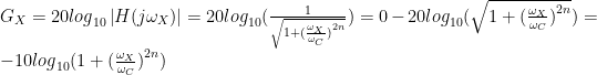
Hence, Passband Gain and Stopband Gain can be determined

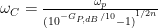
${ G }_{ p,dB }=-10{ log }_{ 10 }\left| 1+{ (\frac { { \omega }_{ P } }{ { \omega }_{ C } } ) }^{ 2n } \right|$

=> ${ (\frac { { \omega }_{ P } }{ { \omega }_{ C } } ) }^{ 2n }={ 10 }^{ -{ G }_{ p,dB }/10 }-1$ ${ \omega }_{ C }=\frac { { \omega }_{ p } }{ { ({ 10 }^{ -{ G }_{ P,dB }/10 }-1) }^{ 1/2n } }$

you can also determine the cutoff frequency this way

${ G }_{ s,dB }=-10{ log }_{ 10 }\left| 1+{ (\frac { { \omega }_{ S } }{ { \omega }_{ C } } ) }^{ 2n } \right|$

=> ${ (\frac { { \omega }_{ S } }{ { \omega }_{ C } } ) }^{ 2n }={ { 10 }^{ -{ G }_{ s,dB }/10 }-1 }$ ${ \omega }_{ C }=\frac { { \omega }_{ S } }{ { ({ 10 }^{ -{ G }_{ S,dB }/10 }-1) }^{ 1/2n } }$

you can also determine the cutoff frequency this way

Dividing the Stopband gain by the Passband gain,

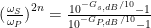
${ (\frac { { \omega }_{ S } }{ { \omega }_{ P } } ) }^{ 2n }=\frac { { { 10 }^{ -{ G }_{ s,dB }/10 }-1 } }{ { { 10 }^{ -{ G }_{ P,dB }/10 }-1 } }$

Rearranging the equation in terms of n so that we can identify the filter order,

$n=\frac { { log }_{ 10 }[({ 10 }^{ -{ G }_{ s,dB }/10 }-1)/({ 10 }^{ -{ G }_{ P,dB }/10 }-1)] }{ 2{ log }_{ 10 }(\frac { { \omega }_{ S } }{ { \omega }_{ P } } ) }$

Example Problem on Butterworth Filter

Design a Butterworth filter with the following specifications

${ G }_{ P,dB }=-3$
${ \omega }_{ P }=20$
${ G }_{ S,dB }=-25$
${ \omega }_{ S}=50$

Also, find the filter’s transfer function.

$n=\frac { { log }_{ 10 }[({ 10 }^{ -{ G }_{ s,dB }/10 }-1)/({ 10 }^{ -{ G }_{ P,dB }/10 }-1)] }{ 2{ log }_{ 10 }(\frac { { \omega }_{ S } }{ { \omega }_{ P } } ) }$

substituting the particular values

$n=\frac { { log }_{ 10 }[({ 10 }^{ 25/10 }-1)/({ 10 }^{ 3/10 }-1)] }{ 2{ log }_{ 10 }(\frac { 50 }{ 20 } ) }$ $n=\frac { { log }_{ 10 }(316.7) }{ 2{ log }_{ 10 }(2.5) }$

n=3.142

When you get a decimal number always round up, as this will give a better roll off than rounding down. We will discuss more about this further down the road.

Now, with the filter order and the filter requirements we can identify the cutoff frequency

We will use both the passband values and stopband values to carry out this calculation

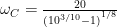
${ \omega }_{ C }=\frac { { \omega }_{ p } }{ { ({ 10 }^{ -{ G }_{ P,dB }/10 }-1) }^{ 1/2n } }$ ${ \omega }_{ C }=\frac { 20 }{ { ({ 10 }^{ 3/10 }-1) }^{ 1/8 } }$ ${ \omega }_{ C }=20.01$

${ \omega }_{ C }=\frac { { \omega }_{ S } }{ { ({ 10 }^{ -{ G }_{ S,dB }/10 }-1) }^{ 1/2n } }$ ${ \omega }_{ C }=\frac { 50 }{ { ({ 10 }^{ 25/10 }-1) }^{ 1/8 } }$ ${ \omega }_{ C }=24.36$

Now, why are there two different values for the same cutoff frequency? Well, we did round off the filter order number for easier design purposes, that’s why!

Let us choose to match up with the passband cutoff frequency and carry on calculating the transfer function taking { \omega }_{ C }=20.01

Next up, we have to design the normalized function before moving on to scaling.

You can either look it up on the Butterworth filter table or you can compute the H(S) using the equation below

$H({ s }_{ n })=\sum _{ k=1 }^{ N/2 }{ \frac { 1 }{ { { s }_{ n } }^{ 2 }+{ b }_{ k }{ s }_{ n }+1 } }$

where ${ b }_{ k }=2sin[\frac { (2k-1)\pi }{ 2N } ]$

but why do all that calculating when you can just copy the numbers from the table. (Don’t worry I’ll show you how to do it in the preceding examples)

So, since N=4 in this case,

Therefore, the coefficients would be a1=2.6131, a2=3.4142, a3=2.6131, a4=1.0000

Putting these coefficients into the normalized transfer function

${ H }_{ n }(s)=\frac { 1 }{ { B }_{ 4 }(s) } =\frac { 1 }{ { s }^{ 4 }+2.6131{ s }^{ 3 }+3.4142{ s }^{ 2 }+2.6131s+1 }$

Now, we are going to scale the normalized function to obtain the actual transfer function,

We’ve got to replace s with s/ ${ \omega }_{ C }$

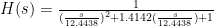
Hence, the final transfer function is

${ H }(s)=\frac { 1 }{ { (\frac { s }{ 20.01 } ) }^{ 4 }+2.6131(\frac { s }{ 20.01 } )^{ 3 }+3.4142(\frac { s }{ 20.01 } )^{ 2 }+2.6131(\frac { s }{ 20.01 } )+1 }$

Frequency response for both values of the cutoff frequency

According to the stopband, the attenuation should be at -25dB, which is the cutoff limit for this filter. Looking at the red curve which depicts the frequency response of the filter if we choose to go with the stopband cutoff frequency, it touches -25dB which is well within the limit. Over attenuation is totally fine too, as long as it does not under attenuate which will allow signals beyond the frequency range to enter. Over attenuation(when the attenuation is less than -25db) will not lead to this problem, so over attenuation and exact attenuation are a thumbs up for your Low Pass Filter. Hence, the blue curve which depicts the frequency response if we choose to go with the passband cutoff frequency over attenuates.

I know the question popping up in your mind right now. If the red curve gives exact attenuation, why not just go with the stopband cutoff frequency?

The problem is with the transition band. At 20 rad/s, the graph should be down by 3dB already but the red curve hardly dipped, it only came down by 1 dB. This is not advisable for the Low Pass Filter. So, the only thing you have to keep in mind is that when choosing the cutoff frequency to scale your transfer function equation, go with the passband cutoff frequency.

Solving Butterworth Filter Transfer Function with Impulse Invariance technique

The Impulse Invariance method does a good job in designing Low Pass Filters. It preserves the order and stability of the analog filter well. However, they cannot be used for High Pass Filters as they are not band limited.

Let us look at the steps involved:

Step 1. Find out the filter specifications

${ G }_{ P }$ is the Pass band gain

Pass band frequency ${ \omega }_{ P }$ ${ G }_{ S }$ is the Stop band gain

Stop band frequency ${ \omega }_{ S }$

Step 2. Find out the order of the filter

$n=\frac { { log }_{ 10 }[({ 10 }^{ -{ G }_{ s,dB }/10 }-1)/({ 10 }^{ -{ G }_{ P,dB }/10 }-1)] }{ 2{ log }_{ 10 }(\frac { { \omega }_{ S } }{ { \omega }_{ P } } ) }$

Step 3. Now, identify the Normalised transfer function, $H({ S }_{ n })$

$H({ S }_{ n })=\sum _{ k=1 }^{ N/2 }{ \frac { 1 }{ { { S }_{ n } }^{ 2 }+{ b }_{ k }{ S }_{ n }+1 } }$

where ${ b }_{ k }=2sin[\frac { (2k-1)\pi }{ 2N } ]$

Step 4. Now, we have to find out the actual transfer function

$H(S)=H({ S }_{ n }){ | }_{ { S }_{ n }=\frac { S }{ { \omega }_{ C } } }$ ${ \omega }_{ C }=\frac { { \omega }_{ S } }{ { [({ \frac { 1 }{ { G }_{ S } } ) }^{ 2 }-1] }^{ 1/2N } }$

Step 5. Now this is the step that determines what method you are using,

we can use a table to do the digital transformation

Type of Transformation	Transformation(Replace s by)
$\frac { 1 }{ s+{ p }_{ i } }$	$\frac { { A }_{ i } }{ 1-{ e }^{ -{ P }_{ i }TZ^{ -1 } } }$
$\frac { (s+a) }{ { (s+a) }^{ 2 }{ +b }^{ 2 } }$	$\frac { 1-{ e }^{ -at }{ (cosbT)z }^{ -1 } }{ 1-{ 2e }^{ -aT }{ (cosbT)z }^{ -1 }{ +e }^{ -2aT }{ z }^{ -2 } }$
$\frac { b }{ { (s+a) }^{ 2 }{ +b }^{ 2 } }$	$\frac { { e }^{ -at }{ (sinbT)z }^{ -1 } }{ 1-{ 2e }^{ -aT }{ (cosbT)z }^{ -1 }{ +e }^{ -2aT }{ z }^{ -2 } }$

How about an example to clear things up?

Solved Example

Butterworth IIR Low Pass Filter using Impulse Invariant Transformation, T=1 sec

$0.707\le \left| H({ e }^{ j\omega }) \right| \le 1.0\quad ;\quad 0\le \omega \le 0.3\pi$ $\left| H({ e }^{ j\omega }) \right| \le 0.2\quad ;\quad 0.75\pi \le \omega \le \pi$

Solution:

1. ${ G }_{ P }$ =0.707[/latex] ${ \omega }_{ P }$ =0.3π[/latex] ${ G }_{ S }$ =0.2[/latex] ${ \omega }_{ S }$ =0.75π[/latex] ${ \omega }_{ P }'$ = $\frac { { \omega }_{ p } }{ T }$ =0.3π/1=o.3×3.14=0.9425[/latex] ${ \omega }_{ S }'$ = $\frac { { \omega }_{ S } }{ T }$ =0.75π/1=2.35624[/latex]

2.Order of the filter

$n=\frac { 1 }{ 2 } \frac { log[\frac { (1/{ (0.2) }^{ 2 })-1 }{ 1/{ (0.707) }^{ 2 })-1 } ] }{ log[\frac { 0.9425 }{ 2.3562 } ] }$

n=1.7339

So rounding this up, our filter order is 2.

3. Next up, according to the steps, we have to find out the normalized function.

$H({ s }_{ n })=\sum _{ k=1 }^{ N/2 }{ \frac { 1 }{ { { s }_{ n } }^{ 2 }+{ b }_{ k }{ s }_{ n }+1 } }$

where ${ b }_{ k }=2sin[\frac { (2k-1)\pi }{ 2N } ]$

k=N/2=2/2=1

${ b }_{ 1 }=2sin\frac { \pi }{ 4 } =1.4142$

Therefore, ${ H(S }_{ n })=\frac { 1 }{ { { s }_{ n } }^{ 2 }{ +1.4142s }_{ n }+1 }$

4. Now, for the actual transfer function

$H(S)={ H(s }_{ n }){ | }_{ { s }_{ n }=\frac { s }{ { \omega }_{ C } } }$

After finding out the cutoff frequency of course,

${ \omega }_{ C }=\frac { { \omega }_{ S } }{ { [({ \frac { 1 }{ { G }_{ S } } ) }^{ 2 }-1] }^{ 1/2N } }$ ${ \omega }_{ C }=\frac { 2.3562 }{ { [({ \frac { 1 }{ 0.2 } ) }^{ 2 }-1] }^{ 1/4 } }$ ${ \omega }_{ C }=\frac { 2.3562 }{ { [({ \frac { 1 }{ 0.2 } ) }^{ 2 }-1] }^{ 1/4 } }$

Ok so now we have the cutoff frequency and we can do the substitution now,

${ H(s }_{ n })=\frac { 1 }{ { (\frac { s }{ 1.0645 } ) }^{ 2 }{ +1.4142(\frac { s }{ 1.0645 } ) }+1 }$

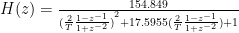
Simplifying this we will obtain the transfer function using impulse invariance method

${ H(s })=\frac { 1.1332 }{ { s }^{ 2 }{ +1.5054s }+1.1332 }$

To perform the digital transform, we need to make sure it is in a form that can be transformed to Z. So we need to make a few changes, starting with completing the square.

${ H(s })=\frac { 1.1332 }{ { (s+0.7527) }^{ 2 }+0.5666 }$ ${ H(s })=\frac { 1.1332 }{ 0.7527 } \times \frac { 0.7527 }{ { (s+0.7527) }^{ 2 }+{ 0.7527 }^{ 2 } }$ ${ H(s })=1.5055\times \frac { 0.7527 }{ { (s+0.7527) }^{ 2 }+{ 0.7527 }^{ 2 } }$

5. Doesn’t this equation look similar to $\frac { b }{ { (s+a) }^{ 2 }{ +b }^{ 2 } }$

So, we will be transforming the equation to $\frac { { e }^{ -at }{ (sinbT)z }^{ -1 } }{ 1-{ 2e }^{ -aT }{ (cosbT)z }^{ -1 }{ +e }^{ -2aT }{ z }^{ -2 } }$ $H(z)=\frac { { e }^{ -at }{ (sinbT)z }^{ -1 } }{ 1-{ 2e }^{ -aT }{ (cosbT)z }^{ -1 }{ +e }^{ -2aT }{ z }^{ -2 } }$ $H(z)=1.5055\times \frac { { e }^{ -0.7527(1) }{ (sin0.7527)z }^{ -1 } }{ 1-{ 2e }^{ -0.7527 }{ (cos0.7527)z }^{ -1 }{ +e }^{ -2(0.7527) }{ z }^{ -2 } }$ $H(z)=1.5055\times \frac { 0.4848{ z }^{ -1 } }{ 1-0.6876{ z }^{ -1 }+0.2219{ z }^{ -2 } }$

Solving Butterworth Filter Transfer Function with Bilinear Transformation technique

Bilinear Transformation is useful when the gains of your filter are constant over certain bands of frequency, such as in Low Pass Filters, High Pass Filters, and Band Pass Filters. The BLT method helps to avoid aliasing of the frequency response that you may encounter while using the Impulse Invariance method to obtain your filter values by mapping one-to-one from the s-plane to the z-plane. Hence, using this method lowers the sampling rate required significantly compared to the IIR method.

This technique involves all the steps in the previous section except the last step and a small change in the second step.

Let us see how with another one of those examples, that’s going to make understanding all this complex stuff a bit easier.

Problem

Design a Butterworth digital IIR highpass filter using Bilinear Transformation by taking T=0.1 second, to satisfy the following specifications.

$0.6\le \left| H({ e }^{ j\omega }) \right| \le 1.0\quad ;\quad 0.7\pi \le \omega \le pi$

$\left| H({ e }^{ j\omega }) \right| \le 0.1\quad ;\quad 0\le \omega \le 0.35\pi$

Solution:

1. For a High Pass Filter

${ G }_{ P }$ =0.6[/latex] ${ \omega }_{ P }$ =0.7π[/latex] ${ G }_{ S }$ =0.1[/latex] ${ \omega }_{ S }$ =0.35π[/latex]

For a Low Pass Filter

${ G }_{ P }$ =0.6

${ \omega }_{ P }$ =0.35π[/latex] ${ G }_{ S }$ =0.1[/latex] ${ \omega }_{ S }$ =0.7π[/latex]

2. Order of the filter

$n=\frac { { log }_{ 10 }[({ 10 }^{ -{ G }_{ s,dB }/10 }-1)/({ 10 }^{ -{ G }_{ P,dB }/10 }-1)] }{ 2{ log }_{ 10 }(\frac { { \Omega }_{ S } }{ { \Omega }_{ P } } ) }$ ${ \Omega }_{ P }=\frac { 2 }{ T } tan\frac { { \omega }_{ P } }{ 2 }$ ${ \Omega }_{ P }=\frac { 2 }{ 0.1 } tan\frac { 0.35\pi }{ 2 }=12.256 rad/sec$ ${ \Omega }_{ S }=\frac { 2 }{ T } tan\frac { { \omega }_{ S } }{ 2 }$ ${ \Omega }_{ S }=\frac { 2 }{ 0.1 } tan\frac { 0.7\pi }{ 2 }=39.2522 rad/sec$ $n=\frac { 1 }{ 2 } \frac { log[\frac { (1/{ (0.1) }^{ 2 })-1 }{ 1/{ (0.6) }^{ 2 })-1 } ] }{ log[\frac { 39.2522 }{ 12.256 } ] }$ $n=\frac { 1 }{ 2 } \frac { log[\frac { 99 }{ 1.7778 } ] }{ log[\frac { 39.2522 }{ 12.256 } ] }$

n=1.726

Therefore, the order of the filter will be 2.

3. Now, for the normalized transfer function

$H({ s }_{ n })=\sum _{ k=1 }^{ N/2 }{ \frac { 1 }{ { { s }_{ n } }^{ 2 }+{ b }_{ k }{ s }_{ n }+1 } }$

where ${ b }_{ k }=2sin[\frac { (2k-1)\pi }{ 2N } ]$

k=N/2=2/2=1

${ b }_{ 1 }=2sin\frac { \pi }{ 4 } =1.4142$ ${ H(s }_{ n })=\frac { 1 }{ { { s }_{ n } }^{ 2 }{ +1.4142s }_{ n }+1 }$

4. Time for the actual transfer function now and we need the cutoff frequency again

${ \omega }_{ C }=\frac { { \omega }_{ S } }{ { [({ \frac { 1 }{ { G }_{ S } } ) }^{ 2 }-1] }^{ 1/2N } }$ ${ \omega }_{ C }=\frac { 39.2522 }{ { [({ \frac { 1 }{ 0.1 } ) }^{ 2 }-1] }^{ 1/4 } }$ ${ \omega }_{ C }=12.44386$ ${ H(s })=\frac { 1 }{ { (\frac { s }{ 12.4438 } ) }^{ 2 }{ +1.4142(\frac { s }{ 12.4438 } ) }+1 }$ ${ H(s })=\frac { 154.849 }{ { s }^{ 2 }{ +17.5955S }+1 }$

5. This is the little twist that I warned y’all about at the beginning, the last step.

So, for this step, we have to replace $s=\frac { 2 }{ T } \frac { 1-{ z }^{ -1 } }{ 1+{ z }^{ -2 } }$

Using the Bilinear Transformation, the transfer function will be

${ H(z })=\frac { 154.849 }{ { (\frac { 2 }{ T } \frac { 1-{ z }^{ -1 } }{ 1+{ z }^{ -2 } } ) }^{ 2 }{ +17.5955(\frac { 2 }{ T } \frac { 1-{ z }^{ -1 } }{ 1+{ z }^{ -2 } } ) }+1 }$

simplifying this very complicated equation, we get

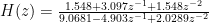
${ H(z })=\frac { { 1.548+3.097 }z^{ -1 }+1.548{ z }^{ -2 } }{ 9.0681-4.903{ z }^{ -1 }+2.0289{ z }^{ -2 } }$

which gives us the transfer function of the High Pass Filter in the ‘z’ domain.

NOTE: When doing calculations on your calculator ensure that the mode is always set to degrees except when you are converting digitally for the impulse invariance method and the bilinear transformation method.

Sources: 1, 2, and 3. The second video is in English (created by Adam Panagos and the other two are in Tamil).