You’ll come across a variety of signals and systems in this digital signal processing course. It might get a bit confusing to remember them all. But eventually, you’ll get a hang of them. You can always keep returning to this post for a quick reference. Here, we have enlisted all the types of signals and systems and the differences between them. Let’s start with some elementary signals that you’ll use quite frequently.
Contents
Elementary Signals
Here is a table of all the different elementary signals, their graphs, and several important properties to take note.
Unit Step Signal

 |
 |
The unit step function is denoted by u(t) or u(n). Since it is UNIT step, the amplitude must be 1.
1) 
2) 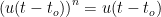
3) u(at)=u(t)
u(at-to )=u(a(t-(to /a)))=u(t-(to /a))
Time scaling is not applicable to a unit step signal.
4)For 
For example, let to=0 be 2. Therefore u(t-2) will be the figure shown below.

Impulse signal

 |
 |
The Unit Impulse Function is given by ????(t) or ????[n].
- ????(n-k) = 1 (for n=k); ????(n-k) = 0 (for n!=k)
- ????(n)=u(n)-u(n-1)
- f(t) ????(t)=f(0)
- ????(t-to)f(t)=f(to)
- ????(-t)=????(t)


Ramp

 |
 |
The Ramp Signal is denoted by r(t)or r(n)
- r(t)=t.u(t)
Therefore,


also, since 


- It is neither an Odd nor an Even Signal
- It is also neither an Energy nor a Power Signal
Parabolic

 |
 |
- It is neither an Odd nor an Even Signal
- It is also neither an Energy nor a Power Signal


Signum
 |
 |
 |
 |
- At t=0, the Signum Signal is discontinuous, Hence, we cannot differentiate this function at 0.
- x(t)=2.u(t)-1
- Can also be represented as


Exponential

 |
 |
 |
- α>0 -> Exponentially Growing; α<0 -> Exponentially Decaying
- When multiplied with unit step signal, it gives only the portion on the graph on the right of they-axis on the exponential graph. If the sign is changed, one has to multiply accordingly.
For example 
multiplied by

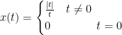
Rectangular
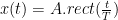
A->Amplitude of Rectangle
T->Period of Rectangle

If given A=5 and T=4
x(t)=5rect(t/4)
Hence, the graph will look like the figure below:

Triangular
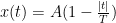
A->Amplitude of the Triangular Signal
T->Time period of the Triangular Signal

If given A=3 and T=5
x(t)=3(1-|t|/5)
Hence, the graph will look like the figure below:

Sinusoidal
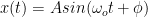
or

A->Amplitude
ωo->Fundamental Frequency
φ->Phase Shift
 |
 |
- ωo=2πf
- f=ωo/2π
- T=1/f=2π/ωo
If given A=1 and ωo=1,
f=1/2π
T=2π
The graph of the signal will be as shown below:

Sinc


Types Of Signals
Signals can be classified in many ways to help one understand the characteristics of the signal they are analyzing
What is the difference between continuous-time and discrete-time signals?
| Continuous-Time Signals | Discrete-Time Signals |
| A Continuous-Time Signal is defined for all values of time. X is the dependent variable and t is the independent variable. When there is an X(t) for every single value of t, it is continuous. | Discrete-Time Signals are defined only at certain discrete values referred to as n and denoted in square brackets. |
| For example, sinusoidal graphs which have a time limit of infinity to negative infinity are clearly continuous-time signals.
|
For example, the graph below is that of a discrete signal

Each time period following 0 can be taken as t1,t2,t3… The difference between these time periods is represented by Δt. If Δt=t1-t0=t2-t1=…, it is uniformly sampled. Since Δt is equal for each point on the time period, we assume Δt=T. That is why the T in x(nT) is cancelled out as all the time period values have a T in them, and the graph is denoted as X[n]. Here ‘n’ is an integer. T is called the ‘sampling period’. |
Discrete values can also be represented within curly braces, where an arrow points at the value when n=0.
 |
What is the difference between deterministic and non-deterministic signals?
| Deterministic signals |
Non-Deterministic signals
|
| A signal is said to be Deterministic when there is no doubt with respect to value at any instant of time. It can be easily identified and represented as a function, X(t). | A signal is said to be Non-Deterministic when it is basically the opposite of that of a Deterministic signal, which means there is uncertainty with respect to value at any instant of time. For example, random signals such as voice signals, there is no fixed pattern as to how it is going to fluctuate and hence it cannot be represented as a function. |
 |
 |
What is the difference between even and odd signals?
| Even Signals | Odd Signals |
| Even signals remain identical when they are reflected or mirrored across the y-axis. | Odd signals are anti-symmetrical when they are reflected or mirrored across the y-axis. |
| For an even signal, x(-t) = x(t) for every value of t. | For an odd signal, x(-t) = -x(t) for every value of t. |
| For example, let us take a sinusoidal signal x(t) = cos(ωt).
x(-t)=cos(-ωt)=cos(ωt)=x(t) Therefore, cos(ωt) is an even signal. |
For example, let us take a sinusoidal signal x(t) = sin(ωt).
x(-t)=sin(-ωt)=-sin(ωt)=-x(t) Therefore, sin(ωt) is an even signal. |
| Similarly, triangular and rectangular signals that have their midpoint at t/n=0 are also examples of even signals | x(t)=t, x(t)=t3 are other examples of odd signals. |
| Sum of two or more even functions, the product of two or more even functions or product of even and odd function results in even function. | For a signal to be odd:
|
What is the difference between periodic and non-periodic signals?
| Periodic Signals | Non-Periodic Signals |
A signal is said to be periodic when it repeats itself for a regular interval of time. When it is periodic, it can be represented as below
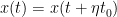
η-> Integer value to->fundamental period which is the smallest positive value of time for which signal is periodic, it may or may not be an integer. (this value cannot be 0 or 2π) |
A signal is said to be non-periodic when it has no pattern, when it does not repeat itself for a regular interval, no matter how large the time interval. The frequency components change over time.
|
| With the fundamental period, we can find the fundamental frequency and the fundamental angular frequency
fo=1/to Cycles per second /Hz ωo=2πfo=2π/to Radians per second |
|
| For example, the sine signal
It has a period of 2π, hence that is the fundamental time period. And it can be represented as sinθ=sin(θ+n2π) where n=0,1,2,… |
Almost all the signals we see in life are non-periodic such as speech signals. |
What is the difference between energy and power signals?
| Energy Signals | Power Signals |
The energy of a signal can be calculated using the formula
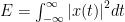 for both periodic and non-periodic signals for both periodic and non-periodic signals |
The power of a signal can be calculated using the formula
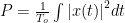 for a periodic signal for a periodic signal for a non-periodic signal for a non-periodic signal |
| Energy of power signal is infinity | Power of energy signal is 0 |
| Majority of the non-periodic signals are energy signals | Majority of the periodic signals are power signals |
| Energy signals are time-limited, they exist only for a short period of time | Power signals are however not time-limited, they exist over an infinite period of time |
What is the difference between real and imaginary signals?
| Real Signals | Imaginary Signals |
| A signal is said to be real when it satisfies condition x(t)=x*(t) | A signal is said to be imaginary when it satisfies condition x(t)=-x*(t) |
| For a real signal imaginary part must be 0 | For an imaginary signal real part must be 0 |
x*(t) means to find the complex conjugate.
You simply have to change the sign of the imaginary part of the complex conjugate.
Types of Systems
A system is a collection of hardware resources that form a device that processes or modifies an input to give an output. A filter can be considered as a system; a signal is sent through the filter, the filter modifies it based on the required frequency and we have the processed output much like the block diagram below.

What is the difference between linear and non-linear systems?
| Linear Systems | Non-Linear Systems |
| A system is said to be linear if it satisfies the superposition principle which is when it satisfies both the Law of Additivity and the Law of Homogeneity. | A system is said to be non-linear if it does not satisfy the Law of Additivity and the Law of Homogeneity and hence the Superposition principle. |
| Law of Additivity:
y1(t)=x1(t) y2(t)=x2(t) y3(t)=x3(t) y’3(t)=y1(t)+y2(t) y3(t)=y’3(t), then it is linear |
For Additivity:
y1(t)=x1(t) y2(t)=x2(t) y3(t)=x3(t) y’3(t)=y1(t)+y2(t) y3(t)≠y’3(t), then it is non-linear |
| For example, system is given by
y(t)=x2(t) y1(t)=x12(t) y2(t)=x22(t) y3(t)=x32(t) y’3(t)=y1(t)+y2(t)= x12(t)+ x22(t) Since y3(t)=y’3(t), the system is linear |
For example, system is given by
y(t)=2t+x(t) y1(t)=2t+x1(t) y2(t)=2t+x2(t) y3(t)=2t+x3(t) y’3(t)=y1(t)+y2(t)=4t+x1(t)+x2(t) Since, y3(t)≠y’3(t), the system is non-linear. |
| Law of Homogeneity:
y(t)=x(t) y(t)–>ky(t) x(t)–>kx(t) if ky(t)=kx(t), then it is linear |
For Homogeneity:
y(t)=x(t) y(t)–>ky(t) x(t)–>kx(t) if ky(t)≠kx(t), then it is non-linear |
| For example, if a system is given by y(t)=x(sin(t))
ky(t)=kx(sin(t)) kx(t)=kx(sin(t)) Since kx(t)=ky(t), the system is linear |
For example, if a system is given by y(t)=2+x(t)
ky(t)=2k+kx(t) Since kx(t)≠ky(t), the system is non-linear |
What is the difference between time-variant and time-invariant systems?
| Time-Variant systems | Time-Invariant systems |
| A system is considered time-variant if its input and output characteristics change with time. You can figure this out by adding a -to and substituting t with t-to. If y(t,to)≠y(t-to), then the system is time-variant. | A system is considered time-invariant if its input and output characteristics do not change with time. You can figure this out by substituting t with to and to-k. If y(t,to)=y(to-k), then the system is time-invariant. |
| For example, given a system
y(t)=2t+x(t) y(t,t0)=2t+x(t-to) y(t-t0)=2(t-to)+x(t-to) Since y(t,to)≠y(t-to), system is time-variant. |
For example, given a system
y(t)=2+x(t) y(t,to)=2+x(t-to) y(t-t0)=2+x(t-to) Since y(t,to)=y(to-k), the system is time-invariant |
What is the difference between linear time-variant and linear time-invariant systems?
| Linear Time-Variant | Linear Time-Invariant |
| A system is said to be Linear Time-Variant when it satisfies both Linearity and Time variance. You can check if it satisfies by conducting the test mentioned above. | A system is said to be Linear Time-Invariant when it satisfies both Linearity and Time variance. You can check if it satisfies by conducting the test mentioned above. |
What is the difference between static and dynamic systems?
| Static (Memoryless) systems | Dynamic (Memory) systems |
| A system is said to be Static when the output of the system depends only on the present values of the input. | A system is said to be Dynamic when the output of the system depends on past or future values of input at any instant of time. |
| when y(t)=x(t), it is considered as present input | When y(t)=x(t-k) where k is any positive real number, it is considered as past input
When y(t)=x(t+k) where k is any positive real number, it is considered as future input |
| Therefore, y(t)=x(t)+2, y(t)=x2(t) are examples of Static systems. | Therefore, y(t)=sin(t), y(t)=x(2t), y(t)=x(t)x(t-1) are examples of Dynamic systems. |
What is the difference between causal and non-causal systems?
| Causal systems | Non-causal systems |
| A system is considered causal if the output response is dependent upon the present and past inputs only. | A system is considered causal if the output response is dependent upon the present and past inputs only. |
| Take note all static systems are causal but not all causal systems are static. | Take note all non-causal systems are dynamic but not all dynamic systems are non-causal |
| For example, given a system y(n)=x(n)+1/x(n-1)
This system depends on the present input, x(n), and the past input, x(n-1). Hence, it is a causal system. |
For example, given a system y(n)=x(n)+1/2x(n+1)
This system depends on the present input, x(n), and the future input, x(n+1). Hence, it is a non-causal system. |
What is the difference between invertible and non-invertible systems?
| Invertible systems | Non-Invertible systems |
| A system is considered invertible if there is a one-to-one mapping between input and output at every instant of time. | A system is considered Non-invertible if a many-to-one mapping exists between the input and the output |
| For example:
y(t)=x(t)+2 where when x is 1, y is 3. When x is 2, y is 4, and so on. Hence, one input can only be mapped to one output. The system is invertible. |
For example:
y(t)=x2(t) where when y is 4, x can be either 2 or -2. The output 4 can be mapped to more than one input. Therefore, the given system is non-invertible. |
What is the difference between stable and unstable systems?
| Stable systems | Unstable systems |
| A system is said to be stable when the output of the system is bounded for a *bounded input at all instants of time, in other words, from infinity to negative infinity. | A system is said to be Unstable when the output of the system is not bounded for a bounded input at all instants of time, in other words from infinity to negative infinity. |
| Examples of bounded signals include unit step signals and sinusoidal signals. | Examples of unbounded signals include exponential signals and y(t)=1/x(t). |
| Given a system y(t)=2x2(t)
let x(t)=u(t), y(t)=2u2(t)=2u(t) u(t) is bounded,and a constant value is also a bounded input. Therefore, y(t) will be a bounded output, and also, a stable system. |
Given a system y(t)=t.x(t) Let x(t)=u(t). y(t)=t.u(t)=r(t) (refer to the table on elementary signals) r(t) is not a bounded input. Hence, the system is unstable. |
Now that we have had a quick revision of all the types of signals and systems, we can get started with the core concepts of this DSP course.
