Fourier series method to design FIR filters

In the designing of an FIR filter, we start from the end that we desire. That is, we begin by plotting a desired/ideal frequency response that we desire from our filter.
Let this desired frequency be H

${ H }_{ d }(\omega )$

We also know that the frequency response of an ideal digital filter is periodic with the period equal to the sampling frequency. And thus, since Fourier series analysis proclaims that any periodic function can be expressed as a linear combination of complex exponentials. Thus, the desired frequency response of our digital filter can be expressed as:

${ H }_{ d }(\omega ){ | }_{ \omega =\omega T }\quad =\quad { H }_{ d }(\omega T)\quad =\quad \sum _{ n=-\infty }^{ \infty }{ { h }_{ d } } (n){ e }^{ -j\omega nT }$

Here T – Sampling time and h(n) – Desired impulse response of the target filter.

Taking inverse DFT we get the desired impulse response (in the frequency domain) as

$\quad { h }_{ d }(n)\quad =\quad { \frac { 1 }{ { \omega }_{ s } } \int _{ \frac { -{ \omega }_{ s } }{ 2 } }^{ \frac { { \omega }_{ s } }{ 2 } }{ { H }_{ d } } }(\omega T){ e }^{ j\omega nT }d\omega$

$h(n)\quad =\quad 0\quad ,\quad \quad otherwise$

However, the impulse response that we obtained above is an infinite duration sequence. But since for an FIR filter, we need to have a system that has a finite impulse response.
To get a finite impulse response from the above equation, we truncate this infinite impulse response to get a finite impulse response sequence of length N, where N is odd.

$h(n)\quad =\quad { h }_{ d }(n)\quad ,\quad \quad for\quad n\quad =\quad -\left( \frac { N-1 }{ 2 } \right) to\quad \left( \frac { N-1 }{ 2 } \right)$

The next step is to get an FIR digital filter’s transfer function (H(z)=Y(z)/X(z)). For this, we have to take the z-transform of the above impulse response equation.
If we had taken the z-transform of the infinite impulse response without truncating it, the result would be the transfer function of an unrealizable non-causal digital filter of infinite duration.
Therefore, taking the z-transform of h(n)

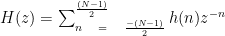
$H(z)=\sum _{ n\quad =\quad \frac { -(N-1) }{ 2 } }^{ \frac { (N-1) }{ 2 } }{ h(n){ z }^{ -n } }$

But due to the presence of positive values of z, this transfer function still represents a non-causal filter.
To get a causal filter, we simply multiply it by the inverse of the positive powers of z.
Therefore:

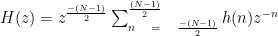
$H(z)={ z }^{ \frac { -(N-1) }{ 2 } }\sum _{ n\quad =\quad \frac { -(N-1) }{ 2 } }^{ \frac { (N-1) }{ 2 } }{ h(n){ z }^{ -n } }$

This modification results in bringing causality to the system. The amplitude response of the filter is not affected.

You can recap the difference between causal and non-causal systems here.

However, the truncation operation of the Fourier series of the impulse response causes oscillation in the pass and stopband. This effect is known as the Gibbs phenomenon.

Gibbs_phenomenon_50 — Unwanted oscillations in passband and stopband (source)

These undesirable oscillations can be reduced by using some special ‘windows’ functions for the truncating process.
Instead of using a sharp window filter like a rectangular window, we can use windows where the values gradually converge to zero.
You can check out the different windowing methods to design FIR filters that address the Gibbs phenomenon here.

Stepwise method to design an FIR filter using Fourier series method

Choose the desired frequency response Hd(ω) of the filter.
Evaluate the Fourier series coefficients of Hd(T). This will give you hd(n) (the target impulse response of the target filter).
Truncate the infinite sequence hd(n) to a finite sequence h(n).
Take Z-transform of h(n) to get a non-causal filter transfer function H(z).
Multiply H(z) by z – (N – 1)/2 to convert the non-causal transfer function to a realizable causal FIR filter transfer function.

Stepwise method to design an FIR filter using Fourier series method

Optical Fiber Comm. Course

Satellite Communication Course

Wireless & Mobile Communication Course