Quantization of filter coefficients in digital filter design

Contents

What is the concept behind the quantization of filter coefficients?

As we have seen often in the course of this Digital Signal Processing course, the design of digital filters involves finding the coefficients of the filter. For computing and evaluating the coefficients of the digital system, we use infinite precision arithmetic. Infinite precision arithmetic is basically when we use numbers whose number of digits is only limited by the available memory of the system. This is done when the speed of calculations is not an issue, but the accuracy is.

Hence, translating that definition of infinite precision arithmetic to DSP systems, we can say that the number of bits that we use in designing a filter is limited by the word length of the register used to the store them.

The fact of the matter, however, is that most of the DSP systems that we use have a fixed number of bits in their registers. The capacity of registers is limited, practically. So how do we fit infinite arithmetic numbers in some finite space?

Easy. We quantize them. Generally, we use quantization methods like rounding or truncating to quantize the filter coefficients to the word size of the register.

The location of poles and zeros of any digital filter directly depends on the value of the filter coefficients. But since we are quantizing the values of the filter coefficients to fit them into the register, there will be a change in the values of the poles and zeros.

This, in turn, causes the location of the poles and zeros to shift from the desired location. Thus the quantization of filter coefficients creates a deviation in the frequency response of the system.

In summary, after quantization, we get a filter that has a frequency response that is different from the frequency response of the filter with unquantized coefficients.

How to reduce the quantization effect on filter coefficients?

We can minimize this drastic effect of quantization on the filter coefficients. The corresponding change in the frequency response can be minimized by realizing a filter with a large number of poles and zeros as an interconnection of second-order sections.

That is, the physical realization of these filters can be done in a particular manner that reduced the effect of the quantization of filter coefficients.

Spoiler! Coefficient quantization has less effect on cascade realization when compared to other realizations.

associative property of convolution — Cascaded systems

Example of the effect of quantization on a filter’s frequency response

Let’s take up a transfer function of a random filter and realize it using direct and cascade forms. We’ll arrive at the conclusion that the shifting of poles and zeros (i.e the frequency response) is closer to the ideally intended filter in the case of cascade realization.

Consider a second-order filter of having a transfer function given by

H(z) = $\frac { 1 }{ (1-0.9{ z }^{ -1 })(1-0.8{ z }^{ -1 }) }$

Direct form realization

We can rearrange the above transfer function to be written as

H(z) = $\frac { { z }^{ 2 } }{ (z-0.9)(z-0.8) }$

Thus, we can see that the poles of the system lie at P1 = 0.9 and P2 = 0.8

Solving the brackets of the original form of the transfer function

H(z) = 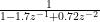$\frac { 1 }{ 1-1.7{ z }^{ -1 }+0.72{ z }^{ -2 } }$

Let’s quantize the coefficients by truncating them to 3-bits.

1.7 $\xrightarrow { Converting\quad to\quad Binary }$ 1.1011 $\xrightarrow { Truncating\quad to\quad 3\quad bits }$ 1.101 $\xrightarrow { Converting\quad to\quad Decimal }$ 2.625

0.72 $\xrightarrow { Converting\quad to\quad Binary }$ 0.1011 $\xrightarrow { Truncating\quad to\quad 3\quad bits }$ 0.101 $\xrightarrow { Converting\quad to\quad Decimal }$ 0.625

Let H'(z) be the transfer function after quantization of coefficients

H'(z) = 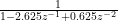$\frac { 1 }{ 1-2.625{ z }^{ -1 }+0.625{ z }^{ -2 } }$

The new poles are at P1′ = 2.625 and P2′ = 0.625

Thus we can see a huge shift in the position of the poles.

Cascade form realization

In the cascade realization method, the transfer function can be written as follows:

H(z) = H1(z) . H2(z)

H1(z) = $\frac { 1 }{ 1-0.9{ z }^{ -1 } }$

H2(z) = $\frac { 1 }{ 1-0.8{ z }^{ -1 } }$

Let’s quantize the coefficients by truncating them to 3-bits.

0.9 $\xrightarrow { Converting\quad to\quad Binary }$ 0.1110 $\xrightarrow { Truncating\quad to\quad 3\quad bits }$ 0.111 $\xrightarrow { Converting\quad to\quad Decimal }$ 0.875

0.8 $\xrightarrow { Converting\quad to\quad Binary }$ 0.1100 $\xrightarrow { Truncating\quad to\quad 3\quad bits }$ 0.110 $\xrightarrow { Converting\quad to\quad Decimal }$ 0.75

The transfer functions after the quantization of coefficients can be written as:

H1′(z) = $\frac { 1 }{ 1-0.875{ z }^{ -1 } }$

H2′(z) = $\frac { 1 }{ 1-0.75{ z }^{ -1 } }$

Thus, we can see that in the cascade form, the deviation of the poles after quantization is less compared to the deviation in direct form. Thus we can say that the effect of quantization is less in cascade form.