Convolution - Derivation, types and properties

Convolution, at the risk of oversimplification, is nothing but a mathematical way of combining two signals to get a third signal. There’s a bit more finesse to it than just that. In this post, we will get to the bottom of what convolution truly is. We will derive the equation for the convolution of two discrete-time signals. Additionally, we will also take a gander at the types of convolution and study the properties of linear convolution.

Contents

What is convolution?

Convolution is a mathematical operation that expresses a relationship between an input signal, the output signal, and the impulse response of a linear-time invariant system.

An impulse response is the response of any system when an impulse signal (a signal that contains all possible frequencies) is applied to it.

As we have seen earlier in this digital signal processing course, a linear time-invariant system is a system that a) behaves linearly, and b) is time-invariant (a shift in time at the input causes a corresponding shift in time in the output). You can understand a bit more about linear time-invariant systems here.

Formula for Convolution of a continuous-time system

y(t) = x(t)*h(t) = 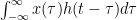$\int _{ -\infty }^{ \infty }{ x(\tau )h(t-\tau )d\tau }$

Formula for Convolution for a discrete-time system

y(n) = x(n)*h(n) = $\sum _{ k=-\infty }^{ \infty }{ x(k)h(n-k) }$

Derivation of the Convolution formula

Consider a relaxed Linear-Time Invariant system (LTI). i.e. A system where when the input x(n) is zero, the output y(n) is zero too.
Apply a unit impulse signal δ(n) to this system. h(n) is the system’s impulse response to this impulse signal. y(n) is the system’s output.

$\delta (n)\quad \longrightarrow \quad y(n)\quad =\quad h(n)$

Since the system is time-invariant, delaying the input by k samples should delay the output by the same amount of samples.

$\delta (n-k)\quad \longrightarrow \quad y(n)\quad =\quad h(n-k)$

Now multiplying both sides by x(k) we get:

$x(k)\delta (n-k)\quad \longrightarrow \quad y(n)\quad =\quad x(k)h(n-k)$

Linear systems satisfy the superposition theorem. And since this system is linear, we can apply summation on both ends.

$\sum _{ k=-\infty }^{ \infty }{ x(k)\delta (n-k) } \quad \longrightarrow \quad y(n)=\sum _{ k=-\infty }^{ \infty }{ x(k)h(n-k) }$

Thus we have

$y(n)=x(n)*h(n)=\sum _{ k=-\infty }^{ \infty }{ x(k)h(n-k) }$

This is called linear convolution. Here is an example that would put things into a visual perspective.

What are the properties of linear convolution?

Linear convolution has three important properties:

Commutative property
Associative property
Distributive property

Commutative property of linear convolution

This property states that linear convolution is a commutative operation. A sample equation would do a better job of explaining the commutative property than any explanation.

x(n)*h(n) = h(n)*x(n)

Associative property of linear convolution

According to the associative property of convolution, we can replace a cascade of Linear-Time Invariant systems in series by a single system whose impulse response is equal to the convolution of the impulse responses of the individual LTI systems.

y(n) = [x(n)*h1(n)]*h2(n) = x(n)*[h1(n)*h2(n)]

Graphically, the associative property of convolution can be represented, as shown below.

Distributive property of linear convolution

The distributive property of linear convolution applies to ‘distributed’ systems. Meaning, if we have two individual Linear-Time Invariant systems with their own individual impulses responses, we can combine them. We can merge them into one LTI system whose impulse response is equal to the sum of the individual responses of the constituent systems. This equation will clear things up a bit.

x(n)*[h1(n)+h2(n)] = [x(n)*h1(n)]+[x(n)*h2(n)]

Graphically this can be represented as shown below.

distributive property of convolution — Distributive property of convolution

What are the types of convolution?

There are two types of convolutions.

Linear Convolution
Circular Convolution

Circular convolution is just like linear convolution, albeit for a few minute differences. When we perform linear convolution, we are technically shifting the sequences. Check the third step in the derivation of the equation. We are delaying both the ends of the equation by k. This graphically translates to linear shifting.

Circular convolution exists for periodic signals. So in a way, when we shift in circular convolution, we keep getting a repeated set of values — kind of like going around a circle. Hence, the name. We have a detailed post on the difference between linear and circular convolutions. Check it out to clarify the concept of circular convolution.