As the size of circuits is growing, the complexity of test pattern generation also increases. Hence manual test generation (being too cumbersome) is not a feasible method anymore. Therefore, we need the help of automatic test pattern generation (ATPG). But methods studied earlier in this DFT course like the path sensitization method is a very intuitive approach and can’t be developed into an algorithm for computer software. The D algorithm is just a derivative of the path sensitization method in a more systematic approach that is suitable for computer acceleration.
The D algorithm was developed by Roth at IBM in 1966 and was the first complete test pattern algorithm designed to be programmable on a computer. The D algorithm is a deterministic ATPG method for combinational circuits, guaranteed to find a test vector if one exists for detecting a fault. It uses cubical algebra for the automatic generation of tests.
Three types of cubes are considered:
- Singular cube
- Propagation D-cube (PDC)
- Primitive D-cube of a fault (PDCF)
Before continuing into cubes, let us focus on an important topic, i.e. D-Algebra.
Contents
The D algebra
The D-algebra is a 5-value logic consisting of logic: 1, 0, D, D', X. The D stands for Discrepancy, as discussed in the path sensitization method.
Following algebraic rules are applicable in D algorithm for intersection:
0 ∩ 0 = 0 ∩ x = x ∩ 0 = 0
1 ∩ 1 = 1 ∩ x = x ∩ 1 = 1
x ∩ x = x
1 ∩ 0 = D
0 ∩ 1 = D’
Note that intersection in D-algebra is quite different to what we are familiar with sets and relations in mathematics. They do not follow properties like commutativity or associativity.
Cubes
Singular Cover
Singular Cover (SC) of any logic gate is the compact form of truth-table. This is done using don’t cares (x). Following reduced truth table is the singular cover of an AND gate.

We know that, for an AND gate, the output is logic-1 only when both of its inputs are high. At the same time, the output is logic-0 for all the other cases where any of its input is low. The output of the AND gate is low for most of the cases. Hence, specifying separate columns for every possible input combinations becomes redundant. Therefore we merge the rows of AND gate and define the truth-table using don’t cares in a more condensed form.
Each row of a singular cover is termed as Singular Cube. The above singular cover of the AND gate has three singular cubes.
Primitive D-cube of a Fault
D-cubes represent the input-output behavior of the good and faulty circuits.
Primitive D-cube of a Fault (PDCF) is used to specify the minimum input conditions required at inputs of a gate to produce an error at its output. This is used for fault activation. PDCF can be derived from the intersection of singular covers of gates in faulty and non-faulty conditions having different outputs.
Example:
Here is an AND gate with s-a-0 fault at the output. To generate the PDCF, we first draw the truth table of the faulty and non-faulty circuit. Next, we derive the singular cover for faulty as well as non-faulty circuits.


For faulty AND gate, the output is always stuck-at-0 independent of its input; hence its singular cover has only one row with inputs (a, b) as don’t cares.
Now, we intersect the singular cubes of the non-faulty and faulty circuits. For PDCF we need to intersect only those columns for which output is different for non-faulty and faulty circuits. Since for faulty circuits, we only have one singular cube {x, x, 0}; we need to intersect it with a singular cube of the non-faulty circuit having the opposite output value (i.e. logic-1). The singular cube {1, 1, 1} perfectly fits this criterion.
{x, x, 0} ∩ {1, 1, 1} = {1 ∩ x, 1 ∩ x, 1 ∩ 0} = {1, 1, D}
Finally, PDCF of this faulty AND gate is {a, b, out} = {1, 1, D}. This is similar to fault excitation we did in the path sensitization method, albeit in a more structured approach.
Here, D is interpreted as being logic-1 if the circuit is fault-free and logic-0 if the fault is present. Notice the order in which the intersection is done! Always intersect as ⇒ singular-cube (non-faulty circuit) ∩ singular-cube (faulty circuit). The reverse will yield different results since the intersection is not commutative and hence will hamper the above interpretation we are trying to opt for.
Propagation D-cube
Propagation D-cubes (PDCs) of a gate causes the output of the gate to depend upon the minimum number of its specified inputs. It is used to propagate D or D’ from a specified input to the output. Propagation D-Cubes can be derived from the intersection of singular cubes of gates of opposite output values.
Example:
Here’s the truth table of an OR gate. To generate the PDC, we find the singular cover for the OR gate.

Now, we intersect the singular cubes of every possible combination(s) with opposite output values. Intersecting the singular cubes of row2 and row1, also row3 and row1 serves the purpose.
{1, x, 1} ∩ {0, 0, 0} = {1 ∩ 0, x ∩ 0, 1 ∩ 0} = {D’, 0, D’}
{x, 1, 1} ∩ {0, 0, 0} = {x ∩ 0, 1 ∩ 0, 1 ∩ 0} = {0, D’, D’}
| a | b | out |
| D’ | 0 | D’ |
| 0 | D’ | D’ |
In this case, the intersection doesn’t need any specific order. If we intersect in the other way, we obtain PDCs as {D, 0, D} and {0, D, D}.
Moreover, there is another option in which we intersect {1, 1, 1} with {0, 0, 0} of the truth table. This yields another possible PDC as {D, D, D} or {D', D', D'}. The following are the complete PDCs of an OR gate.
| a | b | out |
| 0 | D | D |
| D | 0 | D |
| D | D | D |
| 0 | D’ | D’ |
| D’ | 0 | D’ |
| D’ | D’ | D’ |
This is very similar to forward propagation we did in the path sensitization method.
But then why are we learning it? These D-cubes tend to be much more inconvenient and tiresome for us as compared to path sensitization method. The answer is that we human beings have IQ, and hence we can solve methods like path sensitization intuitively. A computer doesn’t the necessary intelligence (yet). The D algorithm takes the creativity out of test generation and allows a computer to do it.
D-cubes of common gates
Singular Cover
| a | b | out |
| 0 | x | 0 |
| x | 0 | 0 |
| 1 | 1 | 1 |
Primitive D-cube of faults
| Fault | a | b | out |
| out→sa0 | 1 | 1 | D |
| out→sa1 | 0 | x | D’ |
| x | 0 | D’ |
Propagation D-cube
| a | b | out |
| 1 | D/D’ | D/D’ |
| D/D’ | 1 | D/D’ |
| D/D’ | D/D’ | D/D’ |
Singular Cover
| a | b | out |
| 0 | 0 | 0 |
| x | 1 | 1 |
| 1 | x | 1 |
Primitive D-cube of faults
| Fault | a | b | out |
| out→sa1 | 0 | 0 | D’ |
| out→sa0 | x | 1 | D |
| 1 | x | D |
Propagation D-cube
| a | b | out |
| 0 | D/D’ | D/D’ |
| D/D’ | 0 | D/D’ |
| D/D’ | D/D’ | D/D’ |
Singular Cover
| a | b | out |
| 0 | x | 1 |
| x | 0 | 1 |
| 1 | 1 | 0 |
Primitive D-cube of faults
| Fault | a | b | out |
| out→sa1 | 1 | 1 | D’ |
| out→sa0 | 0 | x | D |
| x | 0 | D |
Propagation D-cube
| a | b | out |
| 1 | D/D’ | D’/D |
| D/D’ | 1 | D’/D |
| D/D’ | D/D’ | D’/D |
Singular Cover
| a | b | out |
| 0 | 0 | 1 |
| x | 1 | 0 |
| 1 | x | 0 |
Primitive D-cube of faults
| Fault | a | b | out |
| out→sa0 | 0 | 0 | D |
| out→sa1 | x | 1 | D’ |
| 1 | x | D’ |
Propagation D-cube
| a | b | out |
| 0 | D/D’ | D’/D |
| D/D’ | 0 | D’/D |
| D/D’ | D/D’ | D’/D |
Singular Cover
| a | b | out |
| 0 | 0 | 0 |
| 0 | 1 | 1 |
| 1 | 0 | 1 |
| 1 | 1 | 0 |
Primitive D-cube of faults
| Fault | a | b | out |
| out→sa0 | 0 | 1 | D |
| 1 | 0 | D | |
| out→sa1 | 0 | 0 | D’ |
| 1 | 1 | D’ |
Propagation D-cube
| a | b | out |
| 0 | D/D’ | D/D’ |
| D/D’ | 0 | D/D’ |
| D/D’ | 1 | D’/D |
| 1 | D/D’ | D’/D |
Singular Cover
| a | b | out |
| 0 | 0 | 1 |
| 0 | 1 | 0 |
| 1 | 0 | 0 |
| 1 | 1 | 1 |
Primitive D-cube of faults
| Fault | a | b | out |
| out→sa0 | 0 | 0 | D |
| 1 | 1 | D | |
| out→sa1 | 0 | 1 | D’ |
| 1 | 0 | D’ |
Propagation D-cube
| a | b | out |
| 0 | D/D’ | D’/D |
| D/D’ | 0 | D’/D |
| D/D’ | 1 | D/D’ |
| 1 | D/D’ | D/D’ |
Singular Cover
| in | out |
| 0 | 1 |
| 1 | 0 |
Primitive D-cube of faults
| Fault | in | out |
| out→sa0 | 0 | D |
| out→sa1 | 1 | D’ |
Propagation D-cube
| in | out |
| D/D’ | D’/D |
Note that the truth tables of NOT, XOR and XNOR are irreducible; hence their singular cover is the same as their truth-table.
Frontiers
In the D algorithm, we have two essential components:
D-frontier: A set of gates whose output value is currently unknown, but have one or more D (or D’) at their inputs.
J-frontier: A set of gates whose output value is assigned, but input values have not been decided yet.
Check out this part of a combinational circuit for which ATPG is to be performed. The blue gates are D-frontier while green gates are J-frontier.

Test Cubes
A test cube represents partially specified signal values at various nodes in the circuit during each step of the test generation process. Test cubes contain primary inputs as well as internal nodes.
D algorithm ATPG process consists of various steps (we will discuss this in next subheadings). A test cube at ATPG step n is denoted by TC(n).
Intersection of Test Cubes
After every successive step in ATPG, we need to intersect test-cubes to obtain the unified test cube. This intersection is a little different from the former one we studied. In this intersection, two bits can be only intersected if their logic values are not conflicting. The intersection table for the intersection of test-cubes is shown below.
| ∩ | 0 | 1 | x | D | D’ |
| 0 | 0 | 0 | |||
| 1 | 1 | 1 | |||
| x | 0 | 1 | x | D | D’ |
| D | D | D | |||
| D’ | D’ | D’ |
In this table, the empty boxes signify that there is conflict hence no intersection.
For e.g.:
0 ∩ 0 = 0
1 ∩ x = 1
x ∩ D’ = D’
0 ∩ 1 = # (Conflicting)
Implications
Implication in D algorithm means determining unknown values in input/output wires with a known set of values. Implication is done any time a decision is made.
Forward Implication: Uniquely determining the output values from partially (or fully) specified input values of a gate.

Backward Implication: Uniquely determining the un-specified input values from the specified output values (and some input values) of a gate.

Examples
Let us next consider how the various cubes described are used in the D algorithm method to generate a test for a given fault. The test generation process consists of the following three steps:
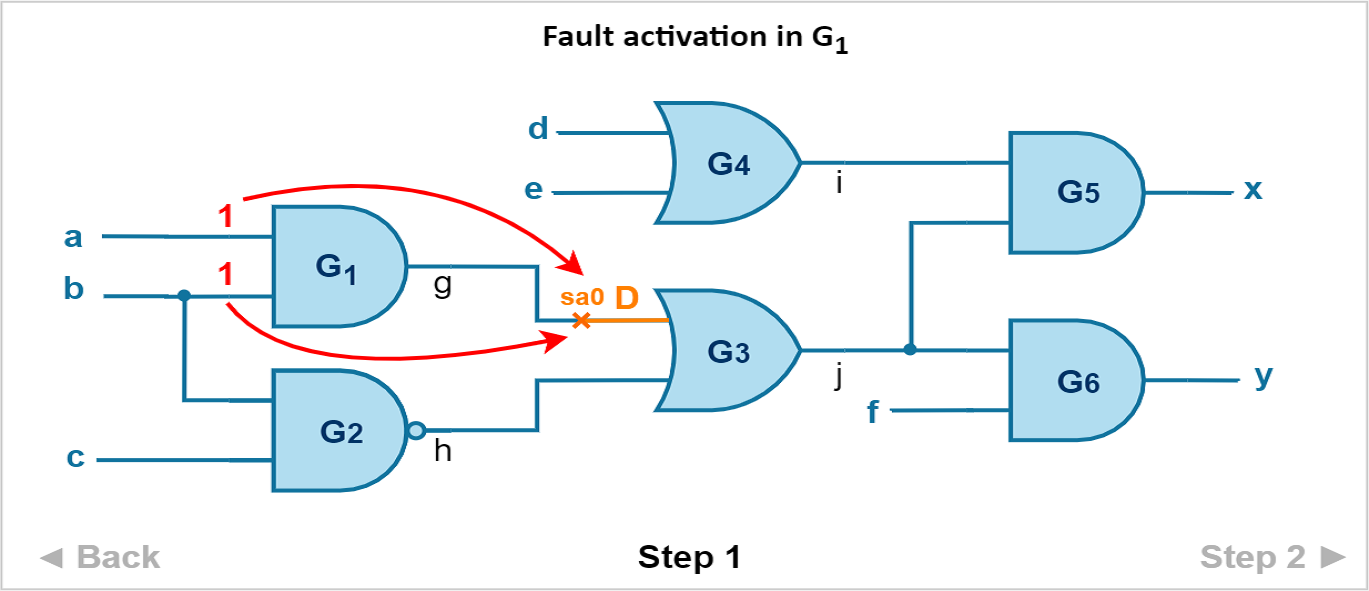
Step 1: Generate a PDCF for the given fault. In this way, we create D-frontier. This is also known as fault activation.
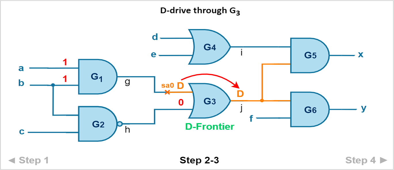
Step 2: Drive the D (or D’) from the output of the gate under test to an output of the circuit by successively intersecting the current test cube with the propagation D-cubes of successive gates. The intersection of a test cube with the propagation D-cube of a successor gate results in another test cube. This process is also known as D-drive or forward propagation.
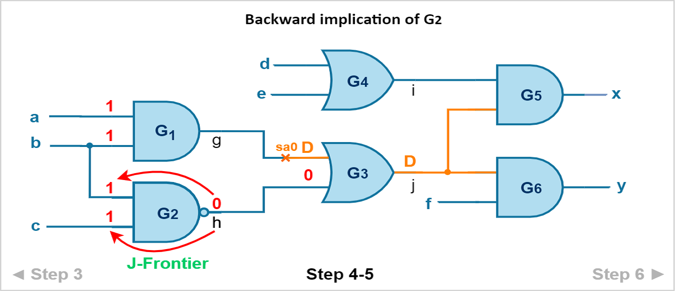
Step 3: Justify the internal line values by driving back towards the inputs of the circuit, assigning input values to the gates so that a consistent set of circuit input values may be obtained. This process is known as justification of J-frontiers or backpropagation.
Step 4: Backtrack to previous steps if any conflict occurs in justification.
Example 1: Fanout free circuit
Let us demonstrate the application of the D algorithm by deriving a test for detecting the g→s-a-0 fault in the following circuit.
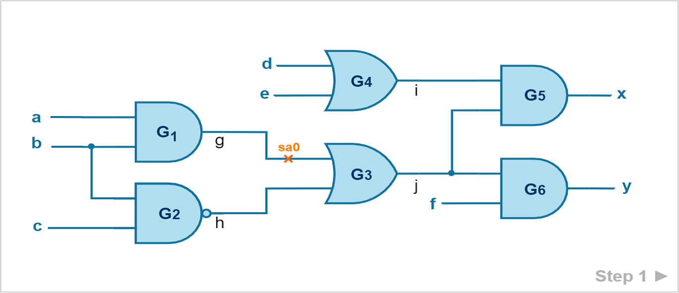
| Step | Operation | a | b | c | d | e | f | g | h | i | j | x | y | Comments |
| 1 | TC(0) = PDCF of G1 | 1 | 1 | D | Fault Activation | |||||||||
| 2 | PDC of G3, PDG3 | D | 0 | D | D-frontier: {G3} | |||||||||
| 3 | TC(1) = TC(0) ∩ PDG3 | 1 | 1 | D | 0 | D | D-Drive through G3 | |||||||
| 4 | Singular Cover SCG2 | 1 | 1 | 0 | ||||||||||
| 5 | TC(2) = TC(1) ∩ SCG2 | 1 | 1 | 1 | D | 0 | D | Backward implication | ||||||
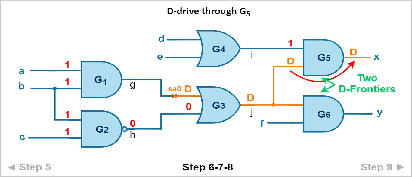
| 6 | TC(2) | 1 | 1 | 1 | D | 0 | D | D-frontier: {G5, G6} | ||||||
| 7 | PDC of G5, PDG5 | 1 | D | D | Choose the path through G5 | |||||||||
| 8 | TC(3) = TC(2) ∩ PDG5 | 1 | 1 | 1 | D | 0 | 1 | D | D | D-drive through G5, D reaches PO | ||||
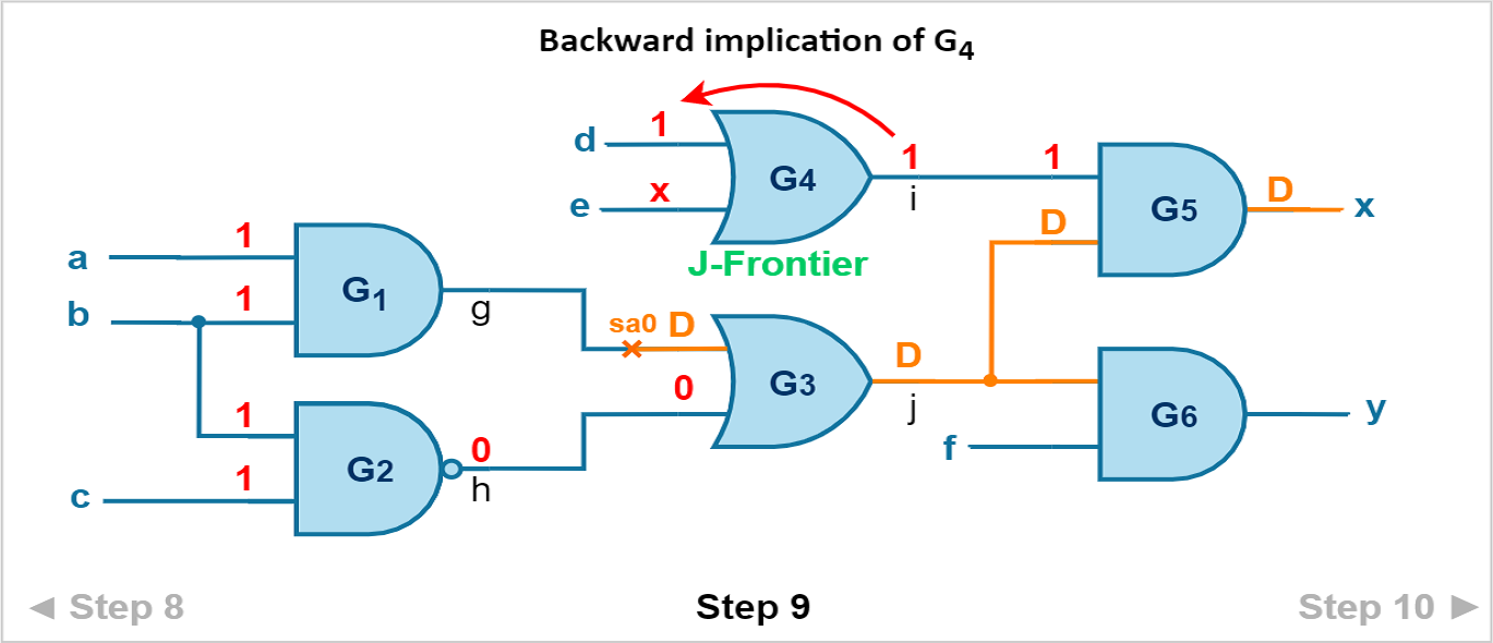
| 9 | Singular Cover SCG5 | 1 | x | 1 | Justification: J-frontier = {G4} | |||||||||
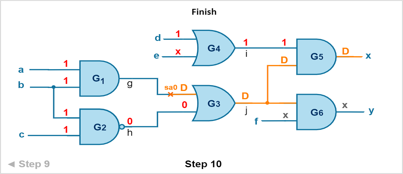
| 10 | TC(4) = TC(3) ∩ SCG5 | 1 | 1 | 1 | 1 | x | x | D | 0 | 1 | D | D | x | Done |
Step 1: Activate the fault by using PDCF of AND gate with output
s-a-0for gate G1. Discrepancy D is generated.Step 2: Forward propagate D by using suitable PDC of OR gate G3. For OR gate we have PDCs as:
{0, D/D’, D/D’},{D/D’, 0, D/D’}and{D/D’, D/D’, D/D’}. Since already one of its input (g) is assigned D, we chose PDC as{D, 0, D}. There is only one single D-frontier in this case.Step 3: Intersect test cubes of row 1 and row 2 to obtain the unified test cube. Follow the test-cube intersection table for this. Empty boxes can be assumed as don’t care (x).
TC(1) = TC(0) ∩ PDG3 = {1, 1, x, x, x, x, D, x, x, x, x, x} ∩ { x, x, x, x, x, x, D, 0, x, D, x, x, x}
= {1∩x, 1∩x, x∩x, x∩x, x∩x, x∩x, D∩D, x∩0, x∩x, x∩D, x∩x, x∩x, x∩x}
= {1, 1, x, x, x, x, D, 0, x, D, x, x, x}
Now we can D-drive through gate G3 towards the next D-frontiers.
Step 4: After every forward propagation, we need to perform backward implication to satisfy the J-frontier and check for consistency. For this, first, obtain the singular cover of NAND gate G2. Since its output is already assigned logic-0, the only possible singular cover is
{1, 1, 0}.Step 5: Intersect test cubes to obtain the unified test cube. J-frontier is satisfied, and consistency is maintained.
Step 6: For forward propagation, there are two possible D-frontiers available, gate G5 and G6. We chose the gate G5.
Step 7: Find PDC of AND gate G5 for forward propagation.
Step 8: D-drive through gate G5 by intersecting the previous two test-cubes. We have finally reached the primary outputs.
Step 9: Perform backward implication to justify the J-frontier gate G4. For this, we again need to find a suitable singular cover.
Step 10: Intersect last two test-cubes to obtain the final test-cube. No conflicts during intersection, hence justification completed. Assign don’t care (x) to the remaining empty boxes like f and y to obtain the complete test-cube.
The test vector for finding the g→s-a-0 fault is:
{a, b, c, d, e, f} = {1, 1, 1, 1, x, x}
Example 2: Reconvergent Fanout circuit
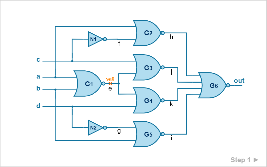
Find a suitable test vector for detecting the e→s-a-0 fault in the following circuit.

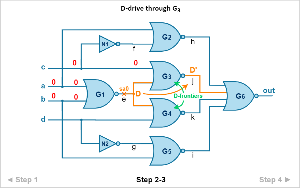

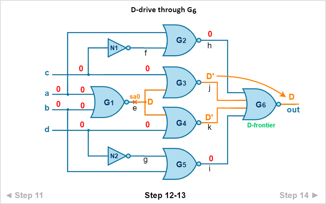

| Step | Operation | a | b | c | d | e | f | g | h | i | j | k | out | Comments |
| 1 | TC(0) = PDCF of G1 | 0 | 0 | D | Fault Activation
D-frontier: {G3, G4} |
|||||||||
| 2 | PDC of G3, PDG3 | 0 | D | D’ | Choose the path through G3 | |||||||||
| 3 | TC(1) = TC(0) ∩ PDG3 | 0 | 0 | 0 | D | D’ | D-Drive through G3 | |||||||
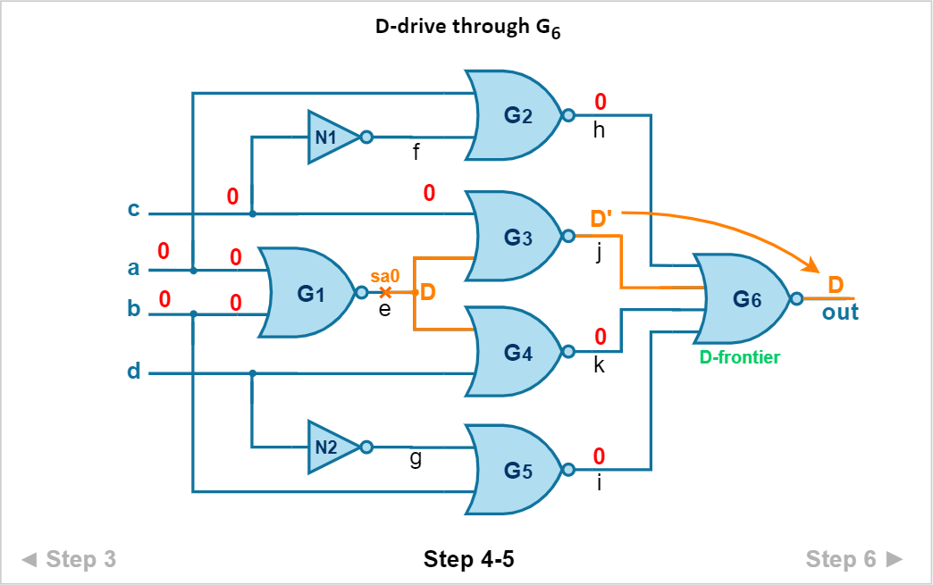
| 4 | PDC of G6, PDG6 | 0 | 0 | D’ | 0 | D | D-frontier: {G6} | |||||||
| 5 | TC(2) = TC(1) ∩ PDG6 | 0 | 0 | 0 | D | 0 | 0 | D’ | 0 | D | D-Drive through G6, D reaches PO | |||
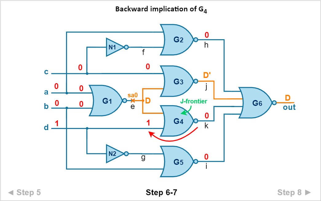
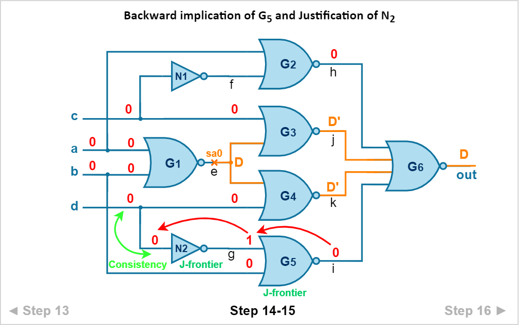
| 6 | Singular Cover SCG4 | 1 | x | 0 | ||||||||||
| 7 | TC(3) = TC(2) ∩ SCG4 | 0 | 0 | 0 | 1 | D | 0 | 0 | D’ | 0 | D | Backward implication of G4 | ||
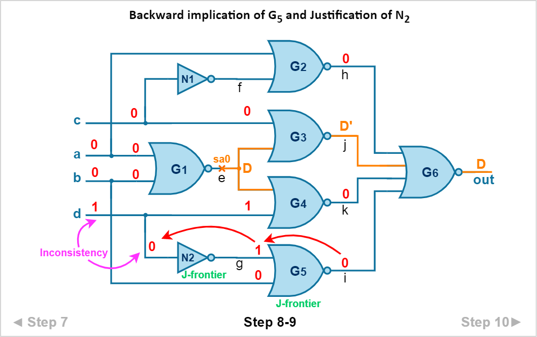
| 8 | Singular Cover SCG5|N2 | 0 | 0 | 1 | 0 | Justification: J-frontier = {N2} | ||||||||
| 9 | TC(4) = TC(3) ∩ SCG5|N2 | 0 | 0 | 0 | # | D | 1 | 0 | 0 | D’ | 0 | D | Consistency Failure | |
| Restart from Step 2 | ||||||||||||||
| 10 | PDC of G3 and G4, PDG3|G4 | 0 | 0 | D | D’ | D’ | Choose both the frontiers: G3 and G4 | |||||||
| 11 | TC(1) = TC(0) ∩ PDG3|G4 | 0 | 0 | 0 | 0 | D | D’ | D’ | D-Drive through G3 and G4 | |||||
| 12 | PDC of G6, PDG6 | 0 | 0 | D’ | D’ | D | D-frontier: {G6} | |||||||
| 13 | TC(2) = TC(1) ∩ PDG6 | 0 | 0 | 0 | 0 | D | 0 | 0 | D’ | D’ | D | D-Drive through G6, D reaches PO | ||
| 14 | Singular Cover SCG5|N2 | 0 | 0 | 1 | 0 | Justification: J-frontier = {N2} | ||||||||
| 15 | TC(3) = TC(2) ∩ SCG5|N2 | 0 | 0 | 0 | 0 | D | 1 | 0 | 0 | D’ | D’ | D | Consistency Success | |
| 16 | Singular Cover SCG2|N1 | 0 | 0 | 1 | 0 | Justification: J-frontier = {N1} | ||||||||
| 17 | TC(4) = TC(3) ∩ SCG5|N1 | 0 | 0 | 0 | 0 | D | 1 | 1 | 0 | 0 | D’ | D’ | D | Consistency Success
Done |
The test vector for finding the e→s-a-0 fault is:
{a, b, c, d} = {0, 0, 0, 0}
In the above example, on step 9, the Justification of the J-frontier N2 fails since the values of test-cubes of step 7 and step 8 conflicts as shown in red colour. This is known as consistency failure, and this is a significant problem in the D algorithm. This is more prevalent with the circuits containing reconvergent fanout. Reconvergent fanout branches are those who again converge later on in next level of the circuit. In this case, the fanout branches emerge via the output of gate G1 and converge later on into G6 inputs.
To solve the consistency failure problem, we need to trace back into earlier stages where we decided of choosing D-frontiers emerging out of fanout branches. Now we need to make a different decision (choose another frontier). In this case, we choose both the frontiers {G3, G4}.
After this decision, we continue the previous steps and find that justification is successful.
This is like a trial-and-error method for computers in which the algorithm keeps changing decision for D-frontiers until all the J-frontiers are satisfied. This is the main drawback of the D algorithm.
Advantages and Disadvantages of D algorithm
D algorithm is a complete ATPG algorithm; hence it guarantees to generate a pattern for a testable fault.
- All the internal signals need to be assigned in the D algorithm, thus it has a huge search space. Therefore, it is a time-consuming and slow algorithm.
- Backtracking is required for consistency checks. Backtracking becomes much more difficult, especially for reconvergent fanout circuits.
D Algorithm Flowchart

D Algorithm Pseudo-code (optional)
The coding of the D algorithm is the job of a VLSI CAD software engineer and hence is out-of-context of this course. However, for the interested folks, following is the snippet of pseudo-code for the D algorithm.
Summary and Conclusion
In this article, we studied one of the very first algorithms for combinational ATPG, i.e., D algorithm. The D algorithm uses a cubical algebra containing singular cover, propagation D-cubes, and primitive D-cubes. The intersection of these cubes with each other yields a test cube. The test cubes represent the partial values of wires assigned during the algorithm. At each progressive step, the previous test cubes need to be intersected with newer test cube.
The D algorithm is all about moving the D-frontier forward towards the primary output (forward propagation or D-drive) while moving the J-frontier backward until we reach the primary inputs (backpropagation or justification).
We saw how reconvergent fanouts create a problem for the algorithm during consistency check. Hence in the next article of the combinational ATPG series, we will discuss other algorithms like PODEM and FAN, where we don’t need to check for consistency.
The D algorithm is still prevalent in the industry today with few modifications and add-ons.
